
Appendix
Applied Structural Equation Modelling for Researchers and Practitioners
ISBN: 978-1-78635-883-7, eISBN: 978-1-78635-882-0
Publication date: 8 December 2016
Citation
Ramlall, I. (2016), "Appendix", Applied Structural Equation Modelling for Researchers and Practitioners, Emerald Group Publishing Limited, Leeds, pp. 131-138. https://doi.org/10.1108/978-1-78635-883-720161027
Publisher
:Emerald Group Publishing Limited
Copyright © 2017 Emerald Group Publishing Limited
A.1 Matrix Operations
Order of a matrix: Number of rows × Number of columns
Matrix addition/subtraction: add/subtract corresponding elements.
Matrix multiplication
(n × p) × (m × n) not workable
Matrix multiplication is associative; that is, A(BC) = (AB)C
Matrix division: A/B = AB −1
To find the inverse of a matrix, there is need to compute the determinant of a matrix (minors and co-factors).
A.2 Determinant of a Matrix
Determinant of a matrix is a number and not a matrix
A.3 Matrix of Minors
To find the minor of each element, just draw a vertical and a horizontal line through that element.
A.4 Matrix of Cofactors
A matrix of cofactors is obtained by multiplying the elements of the matrix of minors by (−1). All odd rows start with a + sign while all even rows
A.5 Transpose of a Matrix
The transpose of a matrix is done by taking the rows of a matrix and placing them into corresponding columns. → A′
A.6 Inverse of a Matrix
The inverse of a matrix, multiplied by itself, generates an identity matrix.
Steps: Minors, Matrix of cofactors, Determinant, Transpose of cofactor matrix and Inverse
A matrix is invertible if its determinant is not zero
If a square matrix is invertible it is called a non-singular matrix
An (n × n) matrix A is invertible if there exists an n × n matrix B such that AB = BA, in this case, B is called the inverse of A.
(Note: Invertible matrices should always be square matrices.)
A.7 Matrix Formulation of SEM
Measurement model (observed–latent):
Structural model (latent–latent):
Y = (Y 1 ,…,Y p )T: (p × 1) vector of observed variables
ω = (ω 1,…,ω q )T: (q × 1) vector of latent variables
µ = an intercept
ɛ j = residual error
η = (q 1 × 1) random vector of dependent latent variables
η = (η 1,…,η q1)T
ξ = (ξ 1,…,ξ q2)T random vector of the explanatory latent variables
ξ = q 2 × 1 [or (q – q 1) × 1] = Number of explanatory latent variables
ω = (n T, ξ T)T
Matrix Notations/Matrix Versions of Eqs. (A.1) and (A.2):
Y: (p × 1) random vector of observed variables
µ: (p × 1) vector of intercepts
˄: (p × q) matrix of factor loadings
ω: (q × 1) matrix of latent variables
ɛ: (p × 1) matrix of measurement errors
η = (q 1 × 1) matrix of dependent latent variables
Γ: (q 1 × q 2) matrix of regression coefficients
ξ = (q 2 × 1) matrix of the explanatory latent variables
δ: (q 1 × 1) matrix of residual errors
When formulating the measurement equation, it is vital to specify the structure of the factor loading matrix, that is which parameters to be made free and which parameters to be made fixed. Such a decision is predominantly based on prior knowledge of the observed and latent variables. The regression coefficients represent the magnitude of the expected changes in the dependent variable for a one-unit change in independent variable.
Measurement equation constitutes a confirmatory tool with a specifically defined loading matrix.
SEM enables researchers to recognize the imperfect nature of their measures by explicitly specifying the error.
Defining the Degrees of Freedom in an SEM Model:
Five variables: Y, X 1, X 2, X 3, Z
Four regression coefficients
Five variances of the independent variables (including the variances of the errors)
Three covariances among the independent variables: defined among the observed independent variables

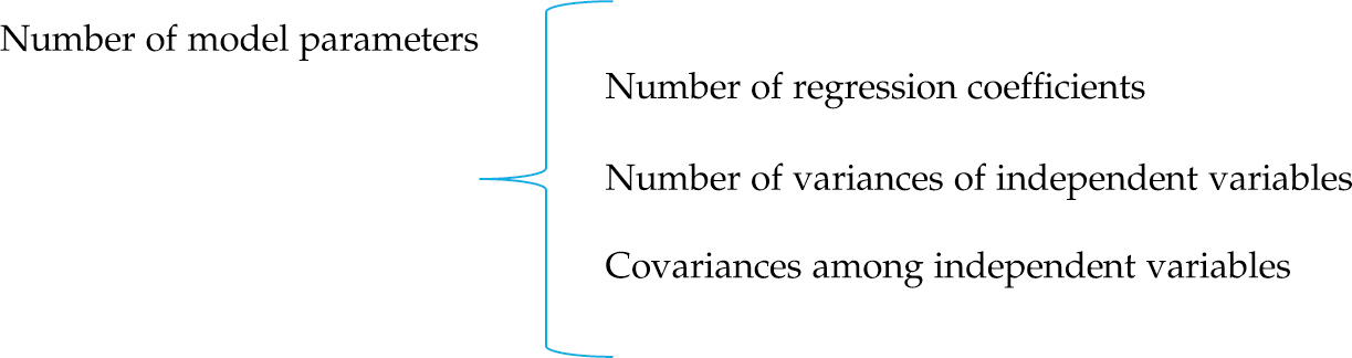
Covariance structure of matrix of SEM will consist of:
Regression coefficients
Variances of the independent variables (including the error variances)
Covariances among the independent variables
All the above will form the model parameters
Degrees of freedom
Number of unique elements
Minus
Order Condition Assessment for Identification:
Number of unique elements in the variance-covariance matrix of the observed variables
minus
Number of parameters to be estimated (Number of regression coefficients, Number of variances and Number of covariances)
The number of regression coefficients is captured by the number of single-headed arrows.
The number of covariances is captured by the number of double-headed arrows.
- Prelims
- 1 Definition of SEM
- 2 Types of SEM
- 3 Benefits of SEM
- 4 Drawbacks of SEM
- 5 Steps in Structural Equation Modelling
- 6 Model Specification: Path Diagram in SEM
- 7 Model Identification
- 8 Model Estimation
- 9 Model Fit Evaluation
- 10 Model Modification
- 11 Model Cross-Validation
- 12 Parameter Testing
- 13 Reduced-Form Version of SEM
- 14 Multiple Indicators Multiple Causes Model of SEM
- 15 Practical Issues to Consider when Implementing SEM
- 16 Review Questions
- 17 Enlightening Questions on SEM
- 18 Applied Structural Equation Modelling Using R
- 19 Applied Structural Equation Modelling using STATA
- Appendix
- About the Author
- Bibliography