
Poverty in the COVID-19 Era: Real-time Data Analysis on Five European Countries
Research on Economic Inequality: Poverty, Inequality and Shocks
ISBN: 978-1-80071-558-5, eISBN: 978-1-80071-557-8
ISSN: 1049-2585
Publication date: 2 December 2021
Abstract
Using real-time data from the University of Luxembourg’s COME-HERE nationally representative panel survey, covering more than 8,000 individuals across France, Germany, Italy, Spain, and Sweden, the author investigates how income distributions and poverty rates have changed from January to September 2020. The author finds that poverty rates increased on average in all countries from January to May and partially recovered in September. The increase in poverty is heterogeneous across countries, with Italy being the most affected and France the least; within countries, COVID-19 contributed to exacerbating poverty differences across regions in Italy and Spain. With a set of poverty measures from the Foster–Greer–Thorbecke family, the author then explores the role of individual characteristics in shaping different poverty profiles across countries. Results suggest that poverty increased disproportionately more for young individuals, women, and respondents who had a job in January 2020 – with different intensities across countries.
Keywords
Citation
Menta, G. (2021), "Poverty in the COVID-19 Era: Real-time Data Analysis on Five European Countries", Bandyopadhyay, S. (Ed.) Research on Economic Inequality: Poverty, Inequality and Shocks (Research on Economic Inequality, Vol. 29), Emerald Publishing Limited, Leeds, pp. 209-247. https://doi.org/10.1108/S1049-258520210000029010
Publisher
:Emerald Publishing Limited
Copyright © 2022 Emerald Publishing Limited
1. Introduction
The COVID-19 pandemic represents an on-going challenge to health systems and economies all over the world. Since its first diffusion in early 2020, the governments of countries most heavily hit by the pandemic have had to design and implement carefully balanced sets of measures and restrictions, with the objective of limiting the diffusion of the virus, while ensuring at least a certain degree of continuity in their countries’ economic activity (Snower, 2020). With economies GDP’s plummeting, space has been given in parallel to recovery schemes, both at the national and transnational levels. An increasing number of papers have documented some of the socio-economic implications of COVID-19, many focusing on its adverse labor market consequences (Adams-Prassl, Boneva, Golin, & Rauh, 2020; Beland, Brodeur, & Wright, 2020; Jones, Philippon, & Venkateswaran, 2020; Jordà, Singh, & Taylor, 2020; Stephany et al., 2020; World Bank, 2020), as well as well as its effects in exacerbating pre-existing inequalities (Adams-Prassl et al., 2020; Ali, Asaria, & Stranges, 2020; Alon, Doepke, Olmstead-Rumsey, & Tertilt, 2020; Blundell, Costa Dias, Joyce, & Xu, 2020; Platt & Warwick, 2020). While worse labor market outcomes are indeed likely to affect household income and its distribution, relatively little is known on about the net distributional and poverty consequences of the combination of confinement measures, higher health hazard, and countercyclical recovery measures and their timeliness.
To the best of my knowledge, this is the first chapter using individual-level longitudinal data to investigate the evolution of poverty in Europe in the COVID-19 era. The majority of the current literature on the poverty and income inequality consequences of COVID-19 relies in fact on microsimulation techniques. Based on different global scenarios of income or consumption contraction, Sumner, Hoy, and Ortiz-Juarez (2020) predict that poverty headcount rates could increase for the first time since the mid-1990s in Europe and Central Asia. Using the EUROMOD microsimulation module on a set of European countries, Almeida et al. (2020) find a 3.6–5.9% reduction in household income and an increase in at-risk-of-poverty (ARP) rates of 1.7 percentage points (from here onwards, pp) in the presence of policy measures. Other papers have used EUROMOD to predict the poverty and inequality consequences of different lockdown scenarios: simulating individuals’ potential wage losses under different lockdown intensities and lengths, Palomino, Rodríguez, and Sebastian (2020) predict an increase of both poverty (3 pp higher headcount ratio under a two-month lockdown) and wage inequality across all European countries. Zooming into the Italian module of EUROMOD, Brunori et al. (2020) predict an increase both in poverty and inequality as a result of the restrictive measures implemented between February and April 2020, and Figari and Fiorio (2020) document an increase in overall income inequality and the ARP between 8 and 15 pp. Using UKMOD, Bronka, Collado, and Richiardi (2020) find that, in an absence of policy changes, a 1.2 pp increase in the poverty rate in the UK can be attributed to the COVID-19 crisis. Simulation and calibration exercises in Li, Vidyattama, La, Miranti, and Sologon (2020) predict that, in absence of policy responses, poverty rates might have doubled in Australia due to COVID-19.
Some exceptions to these simulation exercises on poverty are Brewer and Gardiner (2020), Delaporte, Escobar, and Peña (2020), and Han, Meyer, and Sullivan (2020). Using UK real-time data for 6,000 respondents of the Resolution Foundation’s Coronavirus survey, Brewer and Gardiner (2020) find that 33% of respondents reported a fall in household income between January and May 2020 – evenly distributed across the working-age income distribution. Delaporte et al. (2020) instead look at Latin-American and Caribbean countries, using National Household Survey data harmonized by the Inter-American Development Bank. They find on average a 0.6 pp increase in poverty rates, the largest one being in Peru (1.4 pp). Lastly, Han et al. (2020) use the basic monthly US Current Population Survey (CPS) to show that poverty in the USA fell between February and June 2020, as a result of targeted income-support government policies. However, subsequent waves of the CPS show an increase in poverty rates, in parallel with the higher number of COVID-19 cases confirmed in the USA since the end of the summer.1
I here investigate the evolution of poverty during the first waves of COVID-19 across five European countries, using novel real-time data from the COME-HERE (COVID-19, MEntal HEalth, Resilience, and Self-regulation) longitudinal survey collected by the University of Luxembourg. The survey is nationally representative and follows over 8,000 individuals across France, Germany, Italy, Spain, and Sweden over time (from April 2020, with retrospective information on the pre-lockdown period, up to November 2020). Using poverty measures from the Foster–Greer–Thorbecke (FGT) family (Foster, Greer, & Thorbecke, 1984) and TIP curves, together with relative ARP lines anchored to pre-COVID income distributions, I find that poverty increased ubiquitously across the five countries in analysis during May 2020 with respect to baseline levels measured in January, to almost go back to its initial levels by September. While on average ARP rates increased by 4 pp from January to May, results are heterogenous by country, with Italian residents being the most affected from the COVID-19 crisis (9 pp increase) and French the least (1 pp increase). Recovery patterns from May to September also differ geographically, with only France and Spain experiencing a full recovery and displaying the same poverty figures in January and September. Additionally, I find evidence that the COVID-19 crisis contributed to exacerbating pre-existing geographical differences in poverty rates within the Italian and Spanish territories.
Heterogeneity analysis based on individual characteristics further identifies which categories experienced the higher risk of falling into poverty as a consequence of COVID in May 2020. Poverty measures for individuals below the median age increased more than those of older individuals everywhere; in Spain and Italy, women were disproportionately more vulnerable than men to higher poverty levels. Education and employment, while keeping individuals from experiencing low poverty levels in absolute terms, do not appear to have played a protective role against the relative increase in poverty between January and May: individuals with at least a secondary education degree, as well as those who had a job in January 2020, experienced relatively larger increases in poverty with respect to their counterparts – the educational and employment poverty gaps narrowing as a consequence.
This chapter contributes to the understanding of the evolution of poverty during COVID-19 across different European countries with the use of recent real-time panel data. It further sheds light on the role of individual characteristics in exacerbating or hindering the risk of poverty, by identifying population segments with higher vulnerability to the COVID-19 crisis.
The remainder of the chapter is organized as follows: Section 2 describes the COME-HERE survey and the method used to compute poverty and build the analysis sample. Section 3 presents the main results, together with heterogeneity analysis. Sensitivity analysis is performed in Section 4. Lastly, Section 5 concludes.
2. Data and Methodology
2.1. The COME-HERE Longitudinal Survey
I here use data from the first four waves of the COME-HERE longitudinal survey, conducted by the University of Luxembourg and administered via Qualtrics.2 The survey, aimed at understanding the psychological effects COVID-19 and social distancing measures across Europe, was administered to nationally representative samples of individuals in France, Germany, Italy, Spain, and Sweden for the first time between the end of April and the beginning of May 2020.3 The same pool of individuals was recontacted three additional times in June, August, and end of November/early December 2020. About 8,000 people responded to the first survey wave, evenly distributed across the five different countries.4 About 42% of these respondents were observed in all the next waves as well (with an additional 14% only missing from wave 2); only 17% of respondents in the first wave did not participate to at least another interview.
The COME-HERE survey includes a wide range of questions, spanning from socio-economic and demographic characteristics to a variety of measures of mental health, resilience, and social support. In order to investigate the risk of falling into poverty and the protective role played by socio-demographic factors such as age, gender, and education, I here focus on the economic and demographic dimensions measured by the survey.
In all waves, individuals in the COME-HERE survey were asked, “taking all sources together and all household members living with you,” to recall their net monthly household income (after taxes and transfers) from a few months earlier. In wave 1, which took place between April and May, respondents reported their household income from January 2020; in wave 2, taking place in June, respondents reported their income from April 2020; in wave 3, taking place in August, respondents reported their income from May 2020; lastly, in wave 4, which took place between November and December, respondents were asked about their income in September 2020. Responses were bounded to the seven following income bands: 0–1,250 Euros; 1,250–2,000 Euros; 2,000–4,000 Euros; 4,000–6,000 Euros; 6,000–8,000 Euros; 8,000-12,500 Euros; and >12,500 Euros.5 A “prefer not to say” option was available as an alternative answer.
In order to maximize the observational period of income in the survey and have equally spaced interview windows, I here focus on waves 1, 3, and 4 of the COME-HERE questionnaire. In particular, from wave 1, I derive information on household income in January 2020 and a set of baseline characteristics which are only observed in wave 1 (i.e. age, gender, education, country of residence). From wave 3, I take the reported household income bands referring to the period of May 2020, and from wave 4 household income bands for September 2020.
2.2. Methodology
The household income reported by COME-HERE respondents, as described above, is the starting point to build the measures of poverty used throughout the rest of the chapter. As I here investigate five European economies, I adopt Eurostat’s notion of relative poverty lines, computed as 60% of a country’s median equivalized household income, below which individuals are considered to be at risk of poverty. As in Almeida et al. (2020), in order to avoid confounding in income distributions and relative poverty due to the advancement of the pandemic, I only use pre-COVID-19 income distributions for the definitions of poverty lines in each country (i.e. the January 2020 income distributions from the COME-HERE survey for the main analysis, and then the 2019 EU-SILC wave’s income distributions for sensitivity analysis). Comparing respondents’ equivalized household income with their country’s anchored relative poverty line, I then compute a set of poverty measures of the FGT class (Foster et al., 1984), similar to Delaporte et al. (2020).
In particular, let z denote a country’s relative poverty line and
If α = 0 then the FGT indicator is equal to the headcount ratio p/N, which is informative on the incidence of poverty in a population. For α = 1, then the indicator is equal to the poverty gap ratio, which can be interpreted as the income per capita required to bring every poor at the poverty line and is a measure of poverty intensity. The case proposed by Foster et al. (1984) was using α = 2: here the indicator is referred to as the squared poverty gap, measuring the severity of poverty. Together, these three versions of the index for α = {0, 1, 2} capture the three “i”s of poverty (TIP): incidence, intensity, and inequality. The three dimensions can all be appreciated graphically using TIP curves, which plot cumulative normalized poverty gaps per capita against cumulative population shares (Jenkins & Lambert, 1997). One advantage of using TIP curves, other than the ease of comparison across different income distributions, is that they can be ranked in terms of poverty dominance: given the same poverty line z, if the TIP curve for income distribution x, TIP(x;z), is such that
In order to build national distributions of equivalized household income in the COME-HERE survey, I take the mid-point of the reported household’s banded income for January, May, and September 2020 (as in Clark & Senik, 2010), and divide it by the square root of household size. As reported household sizes are on average larger than official national statistics, I perform some adjustments in order to rule out cohabitation of individuals constituting different households (as it is often the case for young students/workers sharing an apartment with other people without pooling economic resources). In particular, based on their relationship status (single vs in a cohabiting relationship), I attribute household size of one or two to the 534 employed respondents in the sample below 40 years old, with no children, who report having a household size larger than one or two.6 Additionally, in order to avoid an overestimation of poverty for individuals whose household income is in the lowest income band (where the mid-point is automatically below any relative poverty threshold), I treat the 41 individuals living alone, whose employment status is “retired” and who report being in the lowest income band, as non-poor.
The final analysis sample is given by individuals with no missing values for income, household size, and a set of time-invariant individual characteristics described in Table 9.1. In order to avoid the risk of changes in poverty measures over time being driven by non-random attrition between waves 1 and 4, I further restrict the analysis sample to a balanced panel of 4,078 individuals. Descriptive statistics for the estimation sample in Table 9.1 show that, on average, income in the sample fell between January and May, but it slightly raised again in September. Similarly, average ARP rates increased by 4 pp between January and May, to fall again by 3 pp by September. Of the analysis sample, 23% of respondents reside in France, 20% in Germany, 26% in Italy, 25% in Spain, and 6% in Sweden.
Descriptive Statistics for the Analysis Sample.
| Mean | Std. Dev. | Min | Max | |
|---|---|---|---|---|
| Equivalized income (PPP) | ||||
| January 2020 | 2,570.22 | 1,775.77 | 310.48 | 22,354.70 |
| May 2020 | 2,433.25 | 1,698.83 | 287.34 | 23,923.45 |
| September 2020 | 2,439.31 | 1,662.732 | 287.34 | 16,347.45 |
| ARP | ||||
| January 2020 | 0.18 | – | 0 | 1 |
| May 2020 | 0.22 | – | 0 | 1 |
| September 2020 | 0.19 | – | 0 | 1 |
| Time-invariant characteristics | ||||
| Poverty line (PPP) | 1,332.11 | 98.13 | 1,199.7 | 1,489.7 |
| Household size | 3.63 | 1.50 | 1 | 9 |
| Age | 49.49 | 14.58 | 18 | 93 |
| Female | 0.48 | – | 0 | 1 |
| Primary education | 0.19 | – | 0 | 1 |
| Secondary education | 0.37 | – | 0 | 1 |
| Tertiary education | 0.44 | – | 0 | 1 |
| Employed in January 2020 | 0.62 | – | 0 | 1 |
| Resident in France | 0.23 | – | 0 | 1 |
| Resident in Germany | 0.20 | – | 0 | 1 |
| Resident in Italy | 0.26 | – | 0 | 1 |
| Resident in Spain | 0.25 | – | 0 | 1 |
| Resident in Sweden | 0.06 | – | 0 | 1 |
Notes: Descriptive statistics based on the analysis sample (balanced panel of 4,078 individuals across three time periods).
Sample selection statistics presented in Table A1 compare individuals in the estimation sample to the remaining 3,985 respondents who are observed in wave 1. Figures in Table A1 suggest that attrition is indeed non-random: only 18% of respondents in the analysis sample are poor in January 2020, against 24% of all others who are observed in wave 1. Additionally, the analysis sample is made up by individuals who are on average six years older, as well as more likely to be men, in a cohabiting relationship, and with a tertiary education degree. Selection is in place also at the country of residence level: individuals in the sample are 16 pp less likely to be from Sweden, with larger shares of Italian, Spanish, and French residents. While geographic selection might be problematic when interpreting results for Sweden, due to the small number of individuals kept in the sample, selection based on other observable characteristics is less worrying: as individuals who are less likely to be poor are overrepresented in the analysis sample, results could be suffering from an attenuation bias and, as such, should be interpreted as a lower bounds.
With the exception of Table 9.2, results presented in the chapter are based on equivalized disposable income, converted in 2019 USD using purchasing power parity (PPP). Furthermore, results are all weighted for household size – unless otherwise specified.
ARP Rates Across Countries.
| Eurostat (2019) | COME-HERE (January 2020) | |||
|---|---|---|---|---|
| ARP | z | ARP | z | |
| (1) | (2) | (3) | (4) | |
| France | 0.136 | 1,128.1 | 0.167 | 1,039.2 |
| Germany | 0.148 | 1,175.8 | 0.139 | 1,039.2 |
| Italy | 0.201 | 858.3 | 0.211 | 805.0 |
| Spain | 0.207 | 750.8 | 0.196 | 805.0 |
| Sweden | 0.171 | 1,223.7 | 0.131 | 1224.7 |
Notes: Column 1 reports official ARP rates, where the poverty line z reported in column 2 is computed as 60% of the median equivalized income in each country for a one-person household, derived from EU-SILC (Source: Eurostat, 2019). Columns 3 and 4 are based on the COME-HERE survey using the same poverty line definition (here computed on national equivalized household income distributions of respondents in January 2020). Poverty lines in columns 2 and 4 are expressed in euros per month, without any PPP conversion.
3. Results
3.1. Main Results
Before moving on to the main analysis, I first check how reliable the January 2020 ARP rates from the COME-HERE survey are as compared to the official Eurostat ARP statistics for year 2019.7 Column 1 of Table 9.2 reports the Eurostat ARP rates for the five countries in the analysis, computed as the share of individuals whose equivalized disposable income is below their country’s relative poverty lines, and based on EU-SILC data. Relative poverty lines are defined as 60% of the national median equivalized disposable monthly income and are reported in column 2 (expressed in euros per month).8 Using the same definition of ARP rates and poverty lines, but based on the COME-HERE equivalized disposable monthly income distributions, columns 3, and 4 report, respectively, the ARP rates and national relative poverty lines for the analysis sample, in each of the five countries of the analysis. Due to the discrete nature of the reported income in the COME-HERE survey, equivalized household income only takes a fixed set of values, and so do the poverty lines reported in column 4. Nevertheless, poverty lines in column 4 appear to mirror quite closely the ones based on EU-SILC reported in column 2, with absolute differences ranging from only one euro in the case of Sweden, to a maximum of 136.4 euros for Germany. Similarly, ARP rates in column 3 are on average only 0.4 pp lower than the ones in column 1, suggesting that poverty rates in the COME-HERE survey in January 2020 closely mirror representative national statistics from Eurostat in 2019. In the sensitivity analysis (Section 4), I use the Eurostat’s poverty lines in column 2 of Table 9.2, instead of the ones in column 4, in order to assess to what extent results in the chapter are sensitive to the within-sample choice of national relative poverty lines.
The distributions of equivalized disposable monthly income across the countries and periods covered by the analysis sample are displayed in Fig. 9.1. The figure, based on adaptive-kernel densities (Van Kerm, 2003), shows to what extent income distributions across France, Germany, Italy, Spain, and Sweden evolved during different phases of the COVID-19 pandemic. Red vertical lines display national poverty lines, expressed in 2019 USD. Despite equivalized income taking only a discrete number of values, given by combinations of the six income bands and the squared root of household size, I here consider it as being a continuous variable for ease of representation. Bunching around common combinations of income bands and family size is therefore to be expected, and appears to be relatively more common around the poverty thresholds in Italy and Spain. Despite data limitations do not allow us to observe precise income data, the close matching between COME-HERE inequality measures as reported in Clark, D’Ambrosio, and Lepinteur (2020) and Eurostat official statistics on inequality in Europe, as well as Table 9.2 in this chapter, are suggestive evidence that the income distributions observed in COME-HERE are accurate ones. The pattern emerging from Fig. 9.1 confirms the descriptive statistics presented in Table 9.1: with respect to January 2020, income distributions in May appeared to move increasingly to the left, more so for Italy, Spain, and Sweden. Furthermore, all countries experience a shift in population densities in the same time window, with more people reporting equivalized income values below the poverty line. However, by September 2020, income distributions converged back to their January levels – albeit not perfectly, and mostly in Germany and France. As family size is only observed in wave 1, these changes are only driven by variations in reported income and do not reflect demographic changes.

The main results of the chapter are displayed in Table 9.3. The table reports a set of poverty measures across January, May, and September 2020, namely the mean poverty gap among the poor and FGT(α) for α = {0, 1, 2}. Exploiting the additive subgroup decomposability property of the indices, it does so first for the whole analysis sample, and then by country subgroup. Comparing poverty measures for all countries over time, it appears that poverty has progressively worsened from January to May, with the headcount ratio increasing by 4 pp. Not only this is true in terms of incidence (FGT(0), as already suggested by descriptive statistics in Table 9.1, but also according to the intensity and inequality dimensions of poverty. The average normalized poverty gap FGT(1) increased, meaning that poor individuals are on average further away from the poverty line; the higher squared poverty gap FGT(2) suggests a more unequal income distribution below the poverty line. Figures from September 2020 show a recovery from May’s levels, although a partial one.
Poverty Across Countries and Interview Dates (COME-HERE Poverty Lines).
| Mean Gap Among Poor | FGT(0) | FGT(1) (×10) | FGT(2) (×100) | |
|---|---|---|---|---|
| January 2020 | ||||
| All countries | 504.33 | 0.18 | 0.68 | 3.55 |
| France | 477.60 | 0.17 | 0.56 | 2.70 |
| Germany | 481.65 | 0.14 | 0.47 | 2.39 |
| Italy | 453.67 | 0.21 | 0.80 | 4.17 |
| Spain | 551.12 | 0.20 | 0.84 | 4.53 |
| Sweden | 757.24 | 0.13 | 0.66 | 3.86 |
| May 2020 | ||||
| All countries | 518.85 | 0.22 | 0.88 | 4.63 |
| France | 509.08 | 0.18 | 0.66 | 3.32 |
| Germany | 476.59 | 0.17 | 0.56 | 2.79 |
| Italy | 488.55 | 0.29 | 1.17 | 6.27 |
| Spain | 563.07 | 0.24 | 1.06 | 5.69 |
| Sweden | 632.98 | 0.19 | 0.80 | 4.32 |
| September 2020 | ||||
| All countries | 492.20 | 0.19 | 0.72 | 3.71 |
| France | 455.43 | 0.17 | 0.54 | 2.44 |
| Germany | 504.27 | 0.16 | 0.56 | 2.87 |
| Italy | 473.95 | 0.24 | 0.96 | 5.13 |
| Spain | 507.87 | 0.20 | 0.81 | 4.15 |
| Sweden | 639.92 | 0.15 | 0.63 | 3.52 |
Notes: Figures are based on equivalized household disposable income and country-specific COME-HERE poverty lines for the 4,078 respondents in the analysis sample (column 4 of Table 9.2). The mean poverty gap among the poor is expressed in 2019 USD.
Different situations could however be observed in the five countries in the sample. While all countries appear to have suffered a higher poverty intensity, incidence, and inequality from January to May, some recovered faster than others. In France and Spain, under the same FGT(0), FGT(1), and FGT(2) appear to have reached even lower levels in September, as compared to January; Germany, Italy, and Sweden, on the contrary, still displayed higher poverty levels in September than they did at the beginning of the year (with increases in headcount ratios of 2, 3, and 2 pp, respectively).
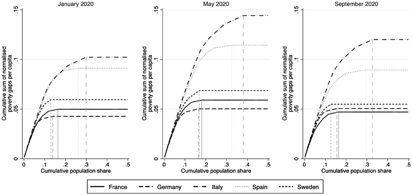
It could be tempting to compare poverty features across countries based on Table 9.3. However, the absence of a unique cross-country poverty line makes it impossible to make any accurate dominance consideration. Fig. 9.2 is an attempt to overcome this limitation, by adopting one unique poverty line based on 60% of the median PPP-adjusted equivalized income of the whole analysis sample in January 2020. The figure plots relative TIP curves in January, May, and September 2020 for all five countries, based on this new universal poverty line of 1,341.28 (in 2019 USD). Headcount ratios, measured as the cumulative population share at which each TIP curve becomes flat, are projected on the x-axes. The intensity of poverty can be seen as the maximum height reached by the curves, and its inequality is given by the slope at which the curves move from the origin to the point where they become flat. The closer one country’s TIP curve is to the poverty worst-case scenario (i.e. a line departing from the origin with slope one), the worse that country is faring in terms of poverty according to its three dimensions. Exact figures on the headcount ratios, poverty gap ratios, and squared poverty gaps from Fig. 9.2 are reported in Table A2 and closely mirror the ones reported in the first panel of Table 9.3 – with the exception of Italy and Spain, where the higher poverty threshold yields larger values for FGT(0), FGT(1), and FGT(2) in January. The poverty ranking suggested by the TIP curves in Fig. 9.2 in January 2020 sees Germany as the least poor of all countries, according to all three dimensions, closely followed by France. Sweden’s TIP distribution, while displaying a lower headcount, stochastically dominates France’s and Germany’s and, as such, fares as the poorest of the three. Italy and Spain are the poorest countries according to all three dimensions, their TIP curves being almost indistinguishable in terms of inequality, but with larger poverty incidence and intensity in Italy. Moving to May 2020, the worsening of poverty makes dominance patterns clearer, without altering the countries’ rankings. However, recovery patterns in September 2020 affected Germany and France’s relative poverty dominance ranking, with France becoming the least poor of all five countries. As compared to January, the final TIP curves in September 2020 see the central and northern European economies becoming more similar to each other in all poverty dimensions, while drifting further away from Spain’s almost constant position. Italy’s TIP curve, on the contrary, is the furthest from its initial position in January, still suffering the economic consequences of the first waves of COVID-19.
The countries in the analysis sample not only differ greatly from each other, but they also encompass very different realities within their own geographical borders. Historical, cultural, and socio-economic backgrounds all contribute to heterogeneity across territorial areas within the same country in experiencing different degrees of poverty and deprivation. Additionally, the role of local governments in the management of pandemic responses might interact with initial geographical pre-dispositions to poverty. The COME-HERE data, providing representative geographical disaggregation at the NUTS 1 level, constitute the perfect tool to further zoom in into geographical decompositions of the poverty consequences of COVID-19. Fig. 9.3 shows the evolution of the headcount ratio over time across the NUTS 1 territorial areas represented in the survey. The figure shows a general increase in poverty rates across most territorial areas in Italy, Spain, and Sweden between January and May. The evolution of poverty across Germany and France appears more nuanced, with the central and western-most regions of Germany being the most visibly affected. Consistent with results from Table 9.3, poverty rates in September are closer to the January ones, although recovery patterns appear to differ from area to area.

While Fig. 9.3 provides a visual representation of the regional evolution of poverty in the countries in the sample, its narrative is sensitive to the choice of poverty thresholds in the legend (here chosen as multiples of 0.05 that were the closest to quintiles of the distribution of poverty across regions). Table A3 provides the level of detail missing in Fig. 9.3, that is, the precise headcount ratios by NUTS 1 and time. While confirming the evidence inferred from Fig. 9.3, Table A3 further identifies a more ubiquitous increase in poverty rates between January and May, with Brandenburg, Niedersachsen, and Sachsen in Germany, and the Est, Sud-Ouest, and Méditerranée regions in France being the only areas where a small decrease was observed instead. Additionally, the table shows that in Italy and Spain pre-existing geographical inequalities in poverty rates were exacerbated as COVID-19 progressed, so that relatively poorest areas such as the South of Spain (Sur) and the Canary Islands, or the Italian South (Sud) and Islands (Isole), were hit the most – with poverty rates reaching almost 40% in May.
3.2. Heterogeneity Analysis: The Role of Individual Characteristics
Other than geography, additional characteristics are likely to play a role in shaping the dynamics of poverty as COVID-19 progresses. Individual factors determined prior to the lockdown, such as age, gender, and employment status in January 2020, can have a protective effect or rather exacerbate the individual risk of falling into poverty. Figs. 9.4–9.8 investigate the evolution of poverty between January and September 2020 in each country by plotting TIP curves across population subgroups. Precise figures on poverty across these subgroups are provided in Appendix Tables A6–A10, reporting population shares, the mean poverty gap for the poor, as well as FGT(0), FGT(1), and FGT (2). Fig. 9.4 first looks at differences by gender. Consistent with official statistics,9 in January 2020 women all over the sample were more likely than man to be at risk of poverty, according to all three dimensions represented by the TIP curves. While the TIP curves changed during the pandemic for both groups, the changes were never large enough to affect the ranking between the two genders, with women being at all times poorer than men. Focusing on differences from January to May, Fig. 9.4 additionally shows an increase in poverty in all countries for both men and women (with the exception of women in Sweden), although with different magnitudes. The increase was disproportionately larger according to all three dimensions of poverty for Spanish and Italian women, the poverty gender gap in May 2020 widening as a result in the two countries. On the contrary, only men become poorer in Sweden, narrowing the poverty gender gap. TIP curves are on average lower in September 2020, with both men and women reaching January’s TIP curve’s level or lower in France, Spain, and Sweden. The recovery from May to September appears to be slower in Italy, especially for men; in Germany, where the TIP curves in all periods are the closest to each other, poverty levels in September appear to be quite close to May’s ones.

Turning to age heterogeneity, Fig. 9.5 shows different pictures across countries in the sample. In January 2020, individuals above the median age of 51 had higher initial levels of poverty in Germany, Italy, and Sweden, and lower levels in France and Spain. Regardless of the departing point, TIP curves of young individuals experienced the highest degree of variability across the sample period – suggesting that they are the group who has suffered the most from the COVID-19 crisis. Despite the higher poverty levels reached in May, September’s TIP curves were back to January levels or lower for all countries – except in Italy and Germany, where the recovery was slower.

Figs. 9.6 and 9.7 show, respectively, whether education (having at least a secondary education degree) and employment (having a job in January 2020) had any protective effects against the risk of poverty in COVID-19 times. From Fig. 9.6, it is clear that the TIP curves of respondents with only a primary education degree always poverty-dominate the curves of more educated individuals. Furthermore, education has a small dampening effect on the higher poverty rates experienced by German and Spanish respondents in May, as compared to January. However, it did not appear to play a protective role against the higher risk of poverty following the beginning of the COVID crisis in the other three countries. Overall, from January to September, the COVID-19 crisis appears to have reduced initial differences in the risk of poverty across educational subgroups for France and Spain, while it contributed to exacerbating those initial differences in the other countries. Similarly to education, Fig. 9.7 shows that individuals who had a job in January 2020 are always less poor than those who did not have a job in all countries in the sample. However, here employment does not play a protective role against the risk of experiencing more severe poverty in May 2020: across all countries, not-employed individuals experienced a relatively small increase in poverty as compared to their fellow employed countrymen. TIP curves for September 2020 reflect this tendency as well: as compared to initial January levels, the recovery from the disproportionately higher increase in poverty rates experienced by employed individuals in May was limited, so that between January and September the poverty gap between employed and not-employed individuals was overall reduced.


3.3. Econometric Analysis
Given the heterogeneity in cross-group poverty trends illustrated above, one may wonder whether the main poverty figures presented in Table 9.3 still hold when keeping constant individual characteristics and geography. Additionally, results presented in Section 3.2 might be at least partly driven by a certain degree of intersectionality between categories – for instance, between education and employment status – so that poverty heterogeneity in one dimension may actually originate from a different one.
I here introduce a simple linear probability model, describing the chance of falling into poverty as a linear function of individual characteristics and time and country fixed effects:
where Poorit is a dummy for individual i having a household equivalized income at time t below their country’s relative poverty line. Xi is a vector of arguably exogenous individual controls: age and its square, education dummies (primary, secondary, or tertiary education), and indicators for being a woman, being in a cohabiting relationship in wave 1, and being employed in January 2020. Wave dummies and country-of-residence dummies are indicated, respectively, by γt and μc; their interaction is γt × μc. Lastly, εit is the error term. I here estimate equation (1) via OLS, with robust standard errors clustered at the individual level.
Fig. 9.8 shows ARP figures across countries and waves based on equation (1). Bars are derived as net effects of the country dummies across time, for the average individual in the estimation sample.10 Fig. 9.8 is consistent with the FGT(0) column of Table 9.3, displaying similar levels and trends in the country-specific ARP rates. The figure shows that, while the increase in poverty rates from January to May is a statistically significant one for all countries but France, a statistically relevant recovery in September was observed only for those countries where the change in poverty rates between January and May was the largest to begin with – namely, Italy, Spain, and Sweden. Finally, September’s poverty levels cannot be ruled out to be identical to January’s ones anywhere other than Italy.

Appendix Table A11 displays regression coefficients for a set of specifications based on equation (1). Column 1 shows OLS estimates for a simplified specification where poverty is regressed only on the time dummies and a constant. Unsurprisingly, the point estimates in column 1 perfectly mirror the change in average headcount ratios over time, as reported in Table 9.3 — the constant’s coefficient here representing the reference period of January 2020. Column 2 further introduces individual characteristics Xi and country dummies μc as controls. No change is observed in the time dummies’ coefficients, suggesting orthogonality between these and the individual characteristics used as controls. Individual characteristics indeed contribute to explaining the risk of poverty, consistently with the differences in the January TIP curves levels observed in Figs. 9.4–9.7. Women and individuals living in Italy or Spain appear to have a higher risk of experiencing poverty across all periods; being in a cohabiting relationship, having at least a secondary education degree, and having a job in January 2020 are instead protective factors against the risk of poverty. In order to assess the evolution of poverty in May and September across different population subgroups, columns 3–6 of Table A11 further augment column 2’s specification by introducing interaction terms between the wave dummies and a set of individual characteristics (these are the same analyzed in Figs. 9.4–9.7, namely gender, age, education, and employment status in January). Keeping all controls constant, only age and employment status appear to be driving statistically significant differences in the average exposure to poverty across subgroups, over January to September. However, given that the median age in the sample is 51, there likely is a high degree of overlap between young individuals and employed individuals – as a large share of individuals above the median age are also in retirement age. This is confirmed by a raw correlation coefficient of 0.43 between the “Below 51 y.o.” and the “Employed in January” dummies. As such, the intersectionality between the two categories might be driving both results in columns 4 and 6. Controlling for all interaction terms at the same time in column 7, only the coefficients of the interactions between “Below 51 y.o.” and the wave dummies attract statistically significant estimates (albeit only in May), while the wave–employment interaction terms cannot be distinguished from zero. Replicating Table A11 using individual fixed-effects regressions instead of pooled OLS yields similar conclusions (results available upon request).
4. Sensitivity Analysis
I here perform a battery of sensitivity tests, in order to assess how robust results presented in Section 3 are to the poverty line specification, the measurement of equivalized income, and sample selection. So far, I computed relative poverty lines based on income distributions in the COME-HERE survey. However, the survey is nationally representative only in terms of gender, region, and age. So it could be the case that income distributions are, for instance, skewed toward the left due to the underreporting of top income values – as it oftentimes is the case in survey data. Furthermore, the incomes reported in the survey are banded, and as such might miss a detailed enough level of variability to make precise inference. Consequently, the COME-HERE national poverty lines displayed in column 4 of Table 9.2 take only three distinct values. For this reason, I now turn to Eurostat relative poverty lines, in order to try and have a more accurate measure of ARP thresholds. Furthermore, Eurostat relative poverty lines are available for two different kinds of households, in order to account for economies of scale across individuals sharing economic resources: a one-person household (displayed in column 1 of Table A4), and a two-adults two-children below 14 years old household (column 4 of Table A4). Using a linear interpolation between the Eurostat poverty lines, I additionally derive the poverty lines in columns 2 and 3, to be used for a two-persons and a three-persons household, respectively.
Results using the high-detailed poverty lines from Table A4 are displayed in Table A5. Comparing the January 2020 FGT(0) figures from Table A5 with official ARP from Table 9.2, it appears that the poverty lines used in Table A5 verge toward an overestimation of the number of people at risk of poverty in the COME-HERE survey. On average, with respect to results from Table 9.3, poverty in Table A5 appears to be more severe in all countries – not only in terms of headcount ratio, but also for the other dimension of poverty. The same considerations hold also for May and September. The only exception is Spain, for which the headcount ratio stayed the same in May and September, while the poverty gap ratio and the squared poverty gap are slightly reduced. Furthermore, the distance between Spain and Italy – the two countries where poverty reached the highest levels during COVID-19 – appears to be larger in Table A5, with the fraction of individuals at risk of poverty in Italy reaching up to 38% in May 2020.11 Qualitatively, the countries’ poverty ranking according to the TIP in May 2020 is the same across Table 9.3 and Table A5.
Another potential concern is related to the measurement of equivalent income. Results presented in Section 3 rely on the definition of household size, which is modified with respect to what is directly reported by respondents as to include considerations on shared housing among individuals constituting different household nuclei. However, these considerations imply normative assumptions on unobserved household types, which may well not be met: for instance, young working adults below the age of 40 with no children who report living with other adult household members, may be taking care of their parents or other relatives instead of sharing their housing with economically independent house-mates. As such, the household size they report would indeed be the correct one and restricting it might induce an underestimation of poverty. Table A12 replicates Table 9.3 using a definition of equivalized household disposable income that does not apply any restrictions to family size as reported by respondents. As expected, what emerges from the table are slightly higher poverty figures throughout the observational window, as compared to those in Table 9.3, with headcount ratios being on average 1 pp larger.
Lastly, I consider whether some of the considerations made so far are sensitive to the inclusion of retired respondents in the analysis sample. Retired respondents might in fact be more protected from the adverse economic consequences of COVID-19 with respect to other individuals, due to their relatively stable pension income flow. In particular, individuals in retirement age are likely to be overrepresented in some groups of the heterogeneity analysis presented in Section 3.2, such as individuals above the median age and individuals who did not have a job in January 2020. Appendix Figs. A1 and A2 address whether results presented in Figs. 9.5 and 9.7 (and their equivalents in Tables A6–A10) are robust to the exclusion of individuals aged 65 years old and above. As compared to Fig. 9.5, results in Fig. A1 (now using 44 as the median age) are qualitatively the same for Germany. However, results for France, Italy, Spain, and Sweden suggest that the poverty rates of older working-age individuals were underestimated for all periods in Fig. 9.5: the gap between old and young individuals is now smaller in Fig. A1, with older respondents’ poverty experience in May being closer to the one of younger respondents.
Moving toward poverty differences across employment status in January 2020, Fig. A2 shows that when excluding individuals above age 65 from the sample the TIP curves of non-employed respondents are on average higher in all periods. However, the relative distance between the TIP curves of employed and non-employed respondents appears to shrink over time in almost all countries, confirming that – even after excluding individuals of retirement age – COVID-19 hit disproportionately more those who had a job in January 2020.
5. Conclusions
The chapter uses real-time longitudinal survey data to describe the evolution of poverty across five European countries – from prior to the diffusion of COVID-19 in Europe, up to September 2020. I find that between January and May poverty rates have increased on average by 4 pp, with significant country-level differences (ranging from 9 pp in Italy to 1 pp in France). By September, poverty rates decreased again – although remaining 1 pp higher than January levels. Consistent with poverty rates, other measures of poverty such as the poverty gap ratio and the squared poverty gap are concordant in identifying an increase, and then a decrease, in all dimensions of poverty. Within-country geographical heterogeneity appears to suggest that the increase in poverty was almost ubiquitous, with few exceptions in France and Germany, and that it contributed to aggravate pre-existing inequalities across regions in Italy and Spain.
Other than geography, individual characteristics play a role in determining individual exposure to poverty: young respondents, women, and those who were employed prior to the spread of the pandemic have born the highest increases in poverty during the first wave of COVID-19, on average.
Some caveats hold when interpreting the results of this chapter. Firstly, non-random attrition of individuals with higher risk of poverty is likely to constitute a source of attenuation bias for the figures presented in the chapter. Additionally, results are restricted to a small set of West-European countries and relatively small sample sizes make it harder to obtain representative estimates of poverty for each subgroup considered in the analysis. Finally, the chapter does not allow to establish a causal link between the evolution of the poverty figures and the COVID-19 crisis per se: in absence of counterfactual scenarios, I am not able to assess to what extent results might have been driven by the health emergency, lockdown-style measures, governments recovery and help schemes, or unobserved confounding factors. Despite the limitations, the chapter provides a compelling first picture of poverty during the pandemic. Results suggest that, while suffering higher poverty levels during the first months of the COVID-19 crisis, governments in France, Germany, Italy, Spain, and Sweden were successful in containing the adverse poverty effects of the pandemics later in the year. Additional evidence would be needed in order to disentangle the role of individual policies and explain cross-countries differences.
Appendix: Other Figures and Tables


Selection in the Analysis Sample (W1): Differences in Means
| Analysis Sample | Rest of W1 Respondents | (1) − (2) | |
|---|---|---|---|
| (1) | (2) | (3) | |
| Equivalized income (PPP) | 2,570.22 | 2,542.01 | 28.22 |
| 1,775.77 | 2,037.90 | 26.53 | |
| ARP | 0.178 | 0.235 | −0.058*** |
| 0.382 | 0.424 | 0.006 | |
| Household size | 3.629 | 3.697 | −0.069*** |
| 1.503 | 1.629 | 0.020 | |
| Age | 49.495 | 42.816 | 6.679*** |
| 14.582 | 17.293 | 0.209 | |
| Female | 0.483 | 0.558 | −0.075*** |
| 0.500 | 0.497 | 0.006 | |
| Cohabiting | 0.717 | 0.602 | 0.114*** |
| 0.451 | 0.489 | 0.006 | |
| Primary education | 0.189 | 0.190 | −0.001 |
| 0.392 | 0.392 | 0.005 | |
| Secondary education | 0.367 | 0.441 | −0.075*** |
| 0.482 | 0.497 | 0.006 | |
| Tertiary education | 0.444 | 0.369 | 0.075*** |
| 0.497 | 0.483 | 0.006 | |
| Employed in January 2020 | 0.618 | 0.528 | 0.090*** |
| 0.486 | 0.499 | 0.006 | |
| Resident in France | 0.232 | 0.182 | 0.050*** |
| 0.422 | 0.386 | 0.005 | |
| Resident in Germany | 0.199 | 0.202 | −0.003 |
| 0.399 | 0.402 | 0.005 | |
| Resident in Italy | 0.255 | 0.205 | 0.050*** |
| 0.436 | 0.404 | 0.005 | |
| Resident in Spain | 0.250 | 0.187 | 0.063*** |
| 0.433 | 0.390 | 0.005 | |
| Resident in Sweden | 0.064 | 0.224 | −0.161*** |
| 0.244 | 0.417 | 0.004 | |
| Observations | 4,078 | 3,985 |
Notes: Odd lines display household size-weighted averages in columns 1 and 2, and differences in means in column 3. Even lines report standard deviations in columns 1 and 2, and standard errors in column 3. W1 indicates wave 1, taking place in April 2020. Other than equivalized income, ARP, and employment status (which are either retrospectively collected or inferred from questions referring to January 2020), all other characteristics refer to April 2020 and are here assumed to be time invariant.
Stars are for standard significance levels: *** p < 0.01, ** p < 0.05, and * p < 0.1.
Poverty Across Countries and Interview Dates (Unique COME-HERE Poverty Line).
| Mean Gap Among Poor | FGT(0) | FGT(1) (×10) | FGT(2) (×100) | |
|---|---|---|---|---|
| January 2020 | ||||
| All countries | 451.83 | 0.22 | 0.73 | 3.73 |
| France | 407.50 | 0.16 | 0.50 | 2.39 |
| Germany | 412.85 | 0.14 | 0.43 | 2.16 |
| Italy | 458.11 | 0.30 | 1.02 | 5.17 |
| Spain | 465.97 | 0.26 | 0.91 | 4.88 |
| Sweden | 616.43 | 0.13 | 0.59 | 3.28 |
| May 2020 | ||||
| All countries | 475.04 | 0.26 | 0.93 | 4.91 |
| France | 438.78 | 0.18 | 0.59 | 2.97 |
| Germany | 407.79 | 0.17 | 0.50 | 2.53 |
| Italy | 507.88 | 0.38 | 1.44 | 7.64 |
| Spain | 472.31 | 0.32 | 1.14 | 6.14 |
| Sweden | 546.12 | 0.17 | 0.69 | 3.60 |
| September 2020 | ||||
| All countries | 443.84 | 0.23 | 0.77 | 3.93 |
| France | 384.90 | 0.16 | 0.47 | 2.13 |
| Germany | 435.47 | 0.16 | 0.51 | 2.61 |
| Italy | 492.25 | 0.33 | 1.20 | 6.27 |
| Spain | 407.86 | 0.29 | 0.89 | 4.52 |
| Sweden | 581.05 | 0.13 | 0.55 | 2.96 |
Notes: Figures are based on equivalized household disposable income of individuals in the analysis sample and a unique COME-HERE poverty line, based on January 2020 incomes from all 4,078 respondents. The mean poverty gap among the poor is expressed in 2019 USD.
ARP Rates by NUTS 1 Areas and Time.
| January | May | September | |
|---|---|---|---|
| France | |||
| Île de France | 0.14 | 0.15 | 0.13 |
| Bassin Parisien | 0.20 | 0.23 | 0.22 |
| Nord - Pas-de-Calais | 0.31 | 0.37 | 0.30 |
| Est | 0.25 | 0.20 | 0.21 |
| Ouest | 0.07 | 0.14 | 0.10 |
| Sud-Ouest | 0.16 | 0.15 | 0.15 |
| Centre-Est | 0.16 | 0.20 | 0.19 |
| Méditerranée | 0.15 | 0.14 | 0.12 |
| Germany | |||
| Baden-Wüttemberg | 0.13 | 0.13 | 0.16 |
| Bayern | 0.08 | 0.10 | 0.09 |
| Berlin | 0.11 | 0.11 | 0.11 |
| Brandenburg | 0.33 | 0.27 | 0.27 |
| Bremen | 0.06 | 0.12 | 0.06 |
| Hamburg | 0.12 | 0.20 | 0.17 |
| Hessen | 0.10 | 0.17 | 0.16 |
| Mecklenburg-Vorpommern | 0.38 | 0.38 | 0.44 |
| Niedersachsen | 0.13 | 0.12 | 0.12 |
| Nordrhein-Westfalen | 0.13 | 0.18 | 0.14 |
| Rheinland-Pfalz | 0.08 | 0.19 | 0.15 |
| Saarland | 0.20 | 0.20 | 0.20 |
| Sachsen | 0.24 | 0.21 | 0.23 |
| Sachsen-Anhalt | 0.19 | 0.23 | 0.23 |
| Schleswig-Holstein | 0.12 | 0.12 | 0.11 |
| Thüringen | 0.21 | 0.28 | 0.30 |
| Italy | |||
| Nord-Ovest | 0.19 | 0.24 | 0.22 |
| Nord-Est | 0.14 | 0.21 | 0.17 |
| Centro (I) | 0.15 | 0.28 | 0.21 |
| Sud | 0.31 | 0.39 | 0.33 |
| Isole | 0.23 | 0.29 | 0.26 |
| Spain | |||
| Noroeste | 0.18 | 0.25 | 0.22 |
| Noreste | 0.19 | 0.22 | 0.17 |
| Comunidad de Madrid | 0.11 | 0.16 | 0.16 |
| Centro (E) | 0.23 | 0.29 | 0.21 |
| Este | 0.18 | 0.19 | 0.17 |
| Sur | 0.23 | 0.30 | 0.26 |
| Canarias | 0.29 | 0.39 | 0.30 |
| Sweden | |||
| Östra Sverige | 0.11 | 0.17 | 0.07 |
| Södra Sverige | 0.11 | 0.19 | 0.17 |
| Norra Sverige | 0.23 | 0.23 | 0.27 |
Notes: Figures are based on equivalized household disposable income of individuals in the analysis sample and country-specific specific COME-HERE poverty lines for the 4,078 respondents in the analysis sample (column 4 of Table 9.2).
ARP Thresholds by Country and Household Type.
| (1) | (2) | (3) | (4) | |
|---|---|---|---|---|
| France | 1,128.08 | 1,541.69 | 1,955.31 | 2,368.92 |
| Germany | 1,175.75 | 1,606.83 | 2,037.92 | 2,469.00 |
| Italy | 858.25 | 1,174.44 | 1,490.64 | 1,806.83 |
| Spain | 750.75 | 1,026.03 | 1,301.30 | 1,576.58 |
| Sweden | 1,223.67 | 1,672.36 | 2,121.06 | 2,569.75 |
Notes: Poverty lines are expressed in euros per month. Columns 1 and 4 reports ARP thresholds from Eurostat for year 2019 for a one-person household and a two-adults two-children household, respectively. Columns 2 and 3 report results from a linear interpolation of the Eurostat poverty lines and are meant to represent ARP thresholds for a two- and a three-persons household, respectively.
Poverty Across Countries and Interview Dates (Eurostat Poverty Lines).
| Mean Gap Among Poor | FGT(0) | FGT (1) (×10) | FGT (2) (×100) | |
|---|---|---|---|---|
| January 2020 | ||||
| All countries | 536.34 | 0.21 | 0.79 | 4.08 |
| France | 604.51 | 0.18 | 0.69 | 3.46 |
| Germany | 613.03 | 0.17 | 0.62 | 3.20 |
| Italy | 457.11 | 0.30 | 1.02 | 5.12 |
| Spain | 520.32 | 0.19 | 0.81 | 4.28 |
| Sweden | 671.22 | 0.16 | 0.70 | 4.05 |
| May 2020 | ||||
| All countries | 560.91 | 0.25 | 1.01 | 5.29 |
| France | 652.13 | 0.19 | 0.79 | 4.15 |
| Germany | 625.64 | 0.19 | 0.73 | 3.78 |
| Italy | 505.85 | 0.38 | 1.44 | 7.59 |
| Spain | 530.27 | 0.24 | 1.02 | 5.38 |
| Sweden | 601.99 | 0.22 | 0.85 | 4.59 |
| September 2020 | ||||
| All countries | 536.80 | 0.22 | 0.84 | 4.30 |
| France | 587.54 | 0.18 | 0.67 | 3.20 |
| Germany | 653.30 | 0.18 | 0.72 | 3.81 |
| Italy | 490.73 | 0.33 | 1.20 | 6.22 |
| Spain | 475.25 | 0.20 | 0.77 | 3.90 |
| Sweden | 591.85 | 0.18 | 0.68 | 3.72 |
Notes: Figures are based on equivalized household disposable income of individuals in the analysis sample and country-specific EU-SILC poverty lines for year 2019, obtained from Eurostat (as displayed in Table A4). The mean poverty gap among the poor is expressed in 2019 USD.
Subgroup Decomposition of Poverty Measures in France.
| Population Share | Mean Gap Among Poor | FGT(0) | FGT(1) (×10) | FGT(2) (×100) | |
|---|---|---|---|---|---|
| January 2020 | |||||
| Male | 0.51 | 475.52 | 0.13 | 0.43 | 2.09 |
| Female | 0.49 | 478.94 | 0.21 | 0.70 | 3.35 |
| Above median age | 0.48 | 374.05 | 0.14 | 0.37 | 1.57 |
| Below median age | 0.52 | 546.13 | 0.19 | 0.74 | 3.74 |
| Not employed in January 2020 | 0.38 | 487.41 | 0.22 | 0.75 | 3.67 |
| Employed in January 2020 | 0.62 | 467.74 | 0.14 | 0.45 | 2.11 |
| Primary education | 0.30 | 517.49 | 0.25 | 0.90 | 4.68 |
| At least secondary education | 0.70 | 444.99 | 0.13 | 0.41 | 1.85 |
| May 2020 | |||||
| Male | 0.51 | 506.02 | 0.14 | 0.49 | 2.47 |
| Female | 0.49 | 510.94 | 0.23 | 0.84 | 4.21 |
| Above median age | 0.48 | 409.24 | 0.15 | 0.43 | 2.01 |
| Below median age | 0.52 | 572.88 | 0.21 | 0.87 | 4.53 |
| Not employed in January 2020 | 0.38 | 484.37 | 0.22 | 0.77 | 3.69 |
| Employed in January 2020 | 0.62 | 530.98 | 0.16 | 0.59 | 3.09 |
| Primary education | 0.30 | 542.64 | 0.26 | 1.00 | 5.33 |
| At least secondary education | 0.70 | 483.68 | 0.15 | 0.51 | 2.45 |
| September 2020 | |||||
| Male | 0.51 | 399.91 | 0.13 | 0.37 | 1.50 |
| Female | 0.49 | 492.18 | 0.21 | 0.71 | 3.42 |
| Above median age | 0.48 | 397.06 | 0.14 | 0.39 | 1.77 |
| Below median age | 0.52 | 494.76 | 0.19 | 0.67 | 3.05 |
| Not employed in Jan 2020 | 0.38 | 458.71 | 0.21 | 0.67 | 3.04 |
| Employed in Jan 2020 | 0.62 | 452.48 | 0.14 | 0.46 | 2.07 |
| Not cohabiting in wave 1 | 0.23 | 555.71 | 0.32 | 1.26 | 6.31 |
| Cohabiting in wave 1 | 0.77 | 375.59 | 0.12 | 0.32 | 1.28 |
| Primary education | 0.30 | 468.23 | 0.24 | 0.79 | 3.80 |
| At least secondary education | 0.70 | 445.59 | 0.14 | 0.43 | 1.85 |
Notes: The table shows subgroup decomposition of poverty measures by gender, age (median age is 51 years old), employment status in January 2020, and education. Figures are based on equivalized household disposable income of individuals in the analysis sample and country-specific specific COME-HERE poverty lines for the 4,078 respondents in the analysis sample (column 4 of Table 9.2).
Subgroup Decomposition of Poverty Measures in Germany.
| Population Share | Mean Gap Among Poor | FGT(0) | FGT(1) (×10) | FGT(2) (×100) | |
|---|---|---|---|---|---|
| January 2020 | |||||
| Male | 0.54 | 431.02 | 0.12 | 0.36 | 1.65 |
| Female | 0.46 | 524.41 | 0.16 | 0.61 | 3.25 |
| Above median age | 0.56 | 492.80 | 0.17 | 0.59 | 3.03 |
| Below median age | 0.44 | 458.20 | 0.10 | 0.33 | 1.57 |
| Not employed in January 2020 | 0.38 | 502.18 | 0.23 | 0.81 | 4.16 |
| Employed in January 2020 | 0.62 | 446.77 | 0.08 | 0.26 | 1.28 |
| Primary education | 0.17 | 440.98 | 0.20 | 0.64 | 2.97 |
| At least secondary education | 0.83 | 495.65 | 0.12 | 0.44 | 2.26 |
| May 2020 | |||||
| Male | 0.54 | 430.31 | 0.14 | 0.43 | 1.96 |
| Female | 0.46 | 515.15 | 0.20 | 0.72 | 3.77 |
| Above median age | 0.56 | 460.48 | 0.19 | 0.61 | 3.12 |
| Below median age | 0.44 | 504.16 | 0.14 | 0.49 | 2.38 |
| Not employed in January 2020 | 0.38 | 482.32 | 0.24 | 0.81 | 4.16 |
| Employed in January 2020 | 0.62 | 469.57 | 0.12 | 0.40 | 1.94 |
| Primary education | 0.17 | 493.20 | 0.23 | 0.82 | 3.96 |
| At least secondary education | 0.83 | 471.19 | 0.15 | 0.50 | 2.55 |
| September 2020 | |||||
| Male | 0.54 | 453.07 | 0.12 | 0.39 | 1.85 |
| Female | 0.46 | 541.90 | 0.19 | 0.75 | 4.06 |
| Above median age | 0.56 | 487.28 | 0.18 | 0.61 | 3.11 |
| Below median age | 0.44 | 533.55 | 0.13 | 0.49 | 2.57 |
| Not employed in January 2020 | 0.38 | 506.10 | 0.24 | 0.86 | 4.48 |
| Employed in January 2020 | 0.62 | 501.65 | 0.10 | 0.37 | 1.86 |
| Primary education | 0.17 | 476.48 | 0.25 | 0.84 | 3.94 |
| At least secondary education | 0.83 | 514.87 | 0.14 | 0.50 | 2.64 |
Notes: The table shows subgroup decomposition of poverty measures by gender, age (median age is 51 years old), employment status in January 2020, and education. Figures are based on equivalized household disposable income of individuals in the analysis sample and country-specific specific COME-HERE poverty lines for the 4,078 respondents in the analysis sample (column 4 of Table 9.2).
Subgroup Decomposition of Poverty Measures in Italy.
| Population Share | Mean Gap Among Poor | FGT(0) | FGT(1) (×10) | FGT(2) (×100) | |
|---|---|---|---|---|---|
| January 2020 | |||||
| Male | 0.50 | 388.06 | 0.16 | 0.52 | 2.53 |
| Female | 0.50 | 493.71 | 0.26 | 1.08 | 5.81 |
| Above median age | 0.39 | 550.79 | 0.18 | 0.83 | 4.49 |
| Below median age | 0.61 | 405.55 | 0.23 | 0.78 | 3.97 |
| Not employed in January 2020 | 0.42 | 532.21 | 0.27 | 1.20 | 6.56 |
| Employed in January 2020 | 0.58 | 363.97 | 0.17 | 0.51 | 2.48 |
| Primary education | 0.15 | 536.10 | 0.29 | 1.30 | 6.77 |
| At least secondary education | 0.85 | 431.40 | 0.20 | 0.71 | 3.70 |
| May 2020 | |||||
| Male | 0.50 | 409.59 | 0.22 | 0.76 | 3.69 |
| Female | 0.50 | 537.90 | 0.35 | 1.58 | 8.84 |
| Above median age | 0.39 | 554.15 | 0.23 | 1.04 | 5.64 |
| Below median age | 0.61 | 459.71 | 0.33 | 1.25 | 6.68 |
| Not employed in January 2020 | 0.42 | 540.96 | 0.33 | 1.47 | 8.08 |
| Employed in January 2020 | 0.58 | 441.76 | 0.26 | 0.96 | 4.99 |
| Primary education | 0.15 | 525.92 | 0.39 | 1.73 | 8.95 |
| At least secondary education | 0.85 | 478.46 | 0.27 | 1.07 | 5.78 |
| September 2020 | |||||
| Male | 0.50 | 449.89 | 0.18 | 0.69 | 3.61 |
| Female | 0.50 | 488.46 | 0.30 | 1.24 | 6.63 |
| Above median age | 0.39 | 548.53 | 0.20 | 0.90 | 4.83 |
| Below median age | 0.61 | 439.92 | 0.27 | 1.01 | 5.31 |
| Not employed in January 2020 | 0.42 | 533.27 | 0.28 | 1.25 | 6.77 |
| Employed in January 2020 | 0.58 | 419.49 | 0.22 | 0.76 | 3.95 |
| Primary education | 0.15 | 548.29 | 0.33 | 1.49 | 7.81 |
| At least secondary education | 0.85 | 454.59 | 0.23 | 0.87 | 4.63 |
Notes: The table shows subgroup decomposition of poverty measures by gender, age (median age is 51 years old), employment status in January 2020, and education. Figures are based on equivalized household disposable income of individuals in the analysis sample and country-specific specific COME-HERE poverty lines for the 4,078 respondents in the analysis sample (column 4 of Table 9.2).
Subgroup Decomposition of Poverty Measures in Spain.
| Population Share | Mean Gap Among Poor | FGT(0) | FGT(1) (×10) | FGT(2) (×100) | |
|---|---|---|---|---|---|
| January 2020 | |||||
| Male | 0.51 | 571.15 | 0.13 | 0.56 | 3.03 |
| Female | 0.49 | 541.30 | 0.27 | 1.14 | 6.12 |
| Above median age | 0.46 | 571.07 | 0.16 | 0.71 | 3.81 |
| Below median age | 0.54 | 539.00 | 0.23 | 0.96 | 5.15 |
| Not employed in January 2020 | 0.37 | 637.56 | 0.24 | 1.17 | 6.57 |
| Employed in January 2020 | 0.63 | 481.12 | 0.17 | 0.65 | 3.32 |
| Primary education | 0.14 | 609.61 | 0.39 | 1.85 | 10.45 |
| At least secondary education | 0.86 | 527.44 | 0.16 | 0.67 | 3.52 |
| May 2020 | |||||
| Male | 0.51 | 555.55 | 0.16 | 0.71 | 3.74 |
| Female | 0.49 | 567.11 | 0.32 | 1.43 | 7.76 |
| Above median age | 0.46 | 546.08 | 0.17 | 0.72 | 3.76 |
| Below median age | 0.54 | 571.35 | 0.30 | 1.35 | 7.36 |
| Not employed in January 2020 | 0.37 | 625.81 | 0.27 | 1.30 | 7.20 |
| Employed in January 2020 | 0.63 | 519.38 | 0.23 | 0.91 | 4.80 |
| Primary education | 0.14 | 620.06 | 0.41 | 1.97 | 11.30 |
| At least secondary education | 0.86 | 544.55 | 0.21 | 0.90 | 4.74 |
| September 2020 | |||||
| Male | 0.51 | 524.07 | 0.14 | 0.56 | 2.82 |
| Female | 0.49 | 499.45 | 0.28 | 1.08 | 5.56 |
| Above median age | 0.46 | 533.97 | 0.16 | 0.65 | 3.36 |
| Below median age | 0.54 | 493.41 | 0.25 | 0.95 | 4.85 |
| Not employed in January 2020 | 0.37 | 563.00 | 0.24 | 1.04 | 5.51 |
| Employed in January 2020 | 0.63 | 466.65 | 0.19 | 0.68 | 3.36 |
| Primary education | 0.14 | 592.12 | 0.36 | 1.65 | 9.08 |
| At least secondary education | 0.86 | 479.36 | 0.18 | 0.67 | 3.32 |
Notes: The table shows subgroup decomposition of poverty measures by gender, age (median age is 51 years old), employment status in January 2020, and education. Figures are based on equivalized household disposable income of individuals in the analysis sample and country-specific COME-HERE poverty lines for the 4,078 respondents in the analysis sample (column 4 of Table 9.2).
Subgroup Decomposition of Poverty Measures in Sweden.
| Population Share | Mean Gap Among Poor | FGT(0) | FGT(1) (×10) | FGT(2) (×100) | |
|---|---|---|---|---|---|
| January 2020 | |||||
| Male | 0.56 | 699.60 | 0.09 | 0.43 | 2.39 |
| Female | 0.44 | 794.09 | 0.18 | 0.97 | 5.74 |
| Above median age | 0.36 | 789.69 | 0.14 | 0.77 | 4.54 |
| Below median age | 0.64 | 735.61 | 0.12 | 0.61 | 3.47 |
| Not employed in January 2020 | 0.28 | 783.81 | 0.31 | 1.62 | 9.54 |
| Employed in January 2020 | 0.72 | 705.66 | 0.06 | 0.29 | 1.65 |
| Primary education | 0.13 | 737.86 | 0.15 | 0.74 | 4.38 |
| At least secondary education | 0.87 | 760.66 | 0.13 | 0.65 | 3.78 |
| May 2020 | |||||
| Male | 0.56 | 589.41 | 0.17 | 0.68 | 3.38 |
| Female | 0.44 | 679.03 | 0.21 | 0.95 | 5.53 |
| Above median age | 0.36 | 686.35 | 0.17 | 0.77 | 4.18 |
| Below median age | 0.64 | 607.92 | 0.20 | 0.82 | 4.41 |
| Not employed in January 2020 | 0.28 | 656.89 | 0.35 | 1.55 | 8.36 |
| Employed in January 2020 | 0.72 | 606.98 | 0.13 | 0.51 | 2.76 |
| Primary education | 0.13 | 654.94 | 0.23 | 1.00 | 5.51 |
| At least secondary education | 0.87 | 628.80 | 0.18 | 0.77 | 4.14 |
| September 2020 | |||||
| Male | 0.56 | 595.00 | 0.11 | 0.44 | 2.32 |
| Female | 0.44 | 671.91 | 0.20 | 0.89 | 5.07 |
| Above median age | 0.36 | 758.51 | 0.14 | 0.74 | 4.30 |
| Below median age | 0.64 | 574.94 | 0.15 | 0.58 | 3.08 |
| Not employed in January 2020 | 0.28 | 662.97 | 0.36 | 1.58 | 9.06 |
| Employed in January 2020 | 0.72 | 592.59 | 0.07 | 0.27 | 1.37 |
| Primary education | 0.13 | 770.57 | 0.26 | 1.33 | 7.92 |
| At least secondary education | 0.87 | 600.88 | 0.13 | 0.53 | 2.85 |
Notes: The table shows subgroup decomposition of poverty measures by gender, age (median age is 51 years old), employment status in January 2020, and education. Figures are based on equivalized household disposable income of individuals in the analysis sample and country-specific specific COME-HERE poverty lines for the 4,078 respondents in the analysis sample (column 4 of Table 9.2).
Poverty Status and Individual Characteristics: OLS Regressions.
| (1) | (2) | (3) | (4) | (5) | (6) | (7) | |
|---|---|---|---|---|---|---|---|
| May 2020 | 0.044*** | 0.044*** | 0.037*** | 0.021*** | 0.039*** | 0.028*** | 0.015 |
| (0.006) | (0.006) | (0.007) | (0.006) | (0.013) | (0.008) | (0.014) | |
| September 2020 | 0.015*** | 0.015*** | 0.011* | 0.005 | 0.011 | 0.005 | −0.003 |
| (0.005) | (0.005) | (0.007) | (0.006) | (0.014) | (0.008) | (0.015) | |
| Female | 0.060*** | 0.052*** | 0.060*** | 0.060*** | 0.060*** | 0.054*** | |
| (0.013) | (0.013) | (0.013) | (0.013) | (0.013) | (0.013) | ||
| Age | 0.007** | 0.007** | 0.007** | 0.007** | 0.007** | 0.007** | |
| (0.003) | (0.003) | (0.003) | (0.003) | (0.003) | (0.003) | ||
| Age2/100 | −0.012*** | −0.012*** | −0.012*** | −0.012*** | −0.012*** | −0.012*** | |
| (0.003) | (0.003) | (0.003) | (0.003) | (0.003) | (0.003) | ||
| Below 51 y.o. | −0.036 | −0.036 | −0.057** | −0.036 | −0.036 | −0.053** | |
| (0.023) | (0.023) | (0.023) | (0.023) | (0.023) | (0.024) | ||
| Cohabiting | −0.122*** | −0.122*** | −0.122*** | −0.122*** | −0.122*** | −0.122*** | |
| (0.014) | (0.014) | (0.014) | (0.014) | (0.014) | (0.014) | ||
| Secondary education | −0.069*** | −0.069*** | −0.069*** | −0.072*** | −0.069*** | −0.068*** | |
| (0.019) | (0.019) | (0.019) | (0.021) | (0.019) | (0.021) | ||
| Tertiary education | −0.146*** | −0.146*** | −0.146*** | −0.150*** | −0.146*** | −0.145*** | |
| (0.018) | (0.018) | (0.018) | (0.020) | (0.018) | (0.020) | ||
| Employed in January | −0.123*** | −0.123*** | −0.123*** | −0.123*** | −0.137*** | −0.131*** | |
| (0.018) | (0.018) | (0.018) | (0.018) | (0.019) | (0.019) | ||
| Resident in Germany | −0.019 | −0.019 | −0.019 | −0.019 | −0.019 | −0.019 | |
| (0.016) | (0.016) | (0.016) | (0.016) | (0.016) | (0.016) | ||
| Resident in Italy | 0.048*** | 0.048*** | 0.048*** | 0.048*** | 0.048*** | 0.048*** | |
| (0.018) | (0.018) | (0.018) | (0.018) | (0.018) | (0.018) | ||
| Resident in Spain | 0.050*** | 0.050*** | 0.050*** | 0.050*** | 0.050*** | 0.050*** | |
| (0.017) | (0.017) | (0.017) | (0.017) | (0.017) | (0.017) | ||
| Resident in Sweden | −0.035 | −0.035 | −0.035 | −0.035 | −0.035 | −0.035 | |
| (0.024) | (0.024) | (0.024) | (0.024) | (0.024) | (0.024) | ||
| May × Female | 0.014 | 0.010 | |||||
| (0.011) | (0.011) | ||||||
| September. × Female | 0.008 | 0.007 | |||||
| (0.011) | (0.011) | ||||||
| May × Below 51 y.o. | 0.042*** | 0.037*** | |||||
| (0.011) | (0.013) | ||||||
| September × Below 51 y.o. | 0.018* | 0.012 | |||||
| (0.011) | (0.013) | ||||||
| May × Secondary edu. | 0.006 | −0.004 | |||||
| (0.014) | (0.015) | ||||||
| September × Secondary edu. | 0.005 | 0.000 | |||||
| (0.015) | (0.016) | ||||||
| May × Empl. in January | 0.025** | 0.011 | |||||
| (0.011) | (0.013) | ||||||
| September × Empl. in January | 0.017 | 0.012 | |||||
| (0.011) | (0.013) | ||||||
| Constant | 0.178*** | 0.404*** | 0.408*** | 0.415*** | 0.407*** | 0.413*** | 0.419*** |
| (0.007) | (0.088) | (0.088) | (0.088) | (0.088) | (0.088) | (0.088) | |
| Observations | 12,234 | 12,234 | 12,234 | 12,234 | 12,234 | 12,234 | 12,234 |
| Adjusted R2 | 0.002 | 0.097 | 0.097 | 0.097 | 0.097 | 0.097 | 0.097 |
Notes: Robust standard errors, clustered at the individual level, in parentheses. The table displays regression coefficients for linear probability models of poverty status on wave dummies (“May 2020” and “September 2020”; January 2020 is the reference category) and controls. Interaction terms between the wave dummies and individual characteristics (gender, age, education, and employment status in January 2020) are displayed at the bottom of the table, in columns 3–7. The wave dummies’ coefficients reported in the first two lines of the table refer to the sample average in columns 1 and 2 and to the interaction terms’ excluded category in columns 3–7.
* p < 0.1, ** p < 0.05, and *** p < 0.01.
Poverty Across Countries and Interview Dates (COME-HERE Poverty Lines).
| Mean Gap Among Poor | FGT(0) | FGT(1) (×10) | FGT(2) (×100) | |
|---|---|---|---|---|
| January 2020 | ||||
| All countries | 512.06 | 0.18 | 0.72 | 3.76 |
| France | 477.03 | 0.18 | 0.59 | 2.84 |
| Germany | 488.67 | 0.15 | 0.53 | 2.68 |
| Italy | 476.69 | 0.21 | 0.85 | 4.53 |
| Spain | 551.72 | 0.20 | 0.85 | 4.57 |
| Sweden | 766.10 | 0.13 | 0.69 | 4.04 |
| May 2020 | ||||
| All countries | 524.63 | 0.23 | 0.92 | 4.90 |
| France | 508.14 | 0.19 | 0.69 | 3.52 |
| Germany | 472.21 | 0.18 | 0.62 | 3.03 |
| Italy | 496.95 | 0.29 | 1.21 | 6.54 |
| Spain | 576.34 | 0.25 | 1.11 | 6.01 |
| Sweden | 657.78 | 0.19 | 0.83 | 4.63 |
| September 2020 | ||||
| All countries | 503.17 | 0.20 | 0.78 | 4.03 |
| France | 456.89 | 0.18 | 0.58 | 2.68 |
| Germany | 495.47 | 0.17 | 0.60 | 3.01 |
| Italy | 495.19 | 0.25 | 1.02 | 5.57 |
| Spain | 523.32 | 0.21 | 0.87 | 4.52 |
| Sweden | 677.12 | 0.15 | 0.68 | 3.88 |
Notes: Figures are based on equivalized household disposable income and country-specific COME-HERE poverty lines for the 4,078 respondents in the analysis sample (column 4 of Table 9.2). Household size is here measured as reported by respondents. The mean poverty gap among the poor is expressed in 2019 USD.
Notes
Poverty figures are available at: http://povertymeasurement.org/covid-19-poverty-dashboard/.
Ethics approval was granted by the Ethics Review Panel of the University of Luxembourg.
Sample representativeness was assured in terms of age, gender, and region of residence.
Each country accounting for around 21% of the observations, with the exception of Sweden which makes up 15% of the first-wave sample.
Income bands in Sweden were expressed in Swedish crowns (SEK) as follows: 0–12,960 SEK; 12,960–20,736 SEK; 20,736–41,472 SEK; 41,472–62,208 SEK; 62,208–82,942 SEK; 82,942–129,597 SEK; and >129,597 SEK.
Section 4 shows that results are not sensitive to the introduction of these restrictions on household size (if anything, poverty figures are underestimated when using them).
Eurostat figures available at: https://ec.europa.eu/eurostat/databrowser/view/tespm010/default/table?lang=en.
The equivalence scale used for Eurostat’s ARP statistics is the OECD-modified scale. Eurostat poverty lines for year 2019 can be accessed here: http://appsso.eurostat.ec.europa.eu/nui/submitViewTableAction.do.
See Eurostat Europe 2020 indicators: https://ec.europa.eu/eurostat/data/database.
Given the panel structure of the data, one may wonder why not estimating a fixed-effects model instead of a pooled OLS one. This is due to the fact that a fixed-effects model would not allow to identify of all the parameters of interest for each country – namely, the coefficients for country dummies μc, their interaction with wave dummies γt, and the constant α.
Italy’s higher poverty rates are mostly driven by data bunching: depending on the wave considered, between 6.6% and 7.4% of Italian respondents have equivalized income of 812.5, which corresponds to individuals living in a four-persons household and reporting an income level between 1,250 and 2,000 euros per month. The COME-HERE poverty threshold (column 4 of Table 9.2) is right below that level of equivalized income (805 euros); Eurostat’s one is right above (858.3 euros).
References
Adams-Prassl, A., Boneva, T., Golin, M., & Rauh, C. (2020). Inequality in the impact of the coronavirus shock: Evidence from real time surveys. Journal of Public Economics, 189, 104245.
Ali, S., Asaria, M., & Stranges, S. (2020). COVID-19 and inequality: Are we all in this together?. Canadian Journal of Public Health, 111, 415–416.
Almeida, V., Barrios, S., Christl, M., De Poli, S., Tumino, A., & van der Wielen, W. (2020). Households’ income and the cushioning effect of fiscal policy measures during the Great Lockdown. Joint Research Centre Working Papers on Taxation and Structural Reforms No. 06/2020.
Alon, T., Doepke, M., Olmstead-Rumsey, J., & Tertilt, M. (2020). The impact of COVID-19 on gender equality. NBER Working Paper No. 26947.
Beland, L. P., Brodeur, A., & Wright, T. (2020). The short-term economic consequences of COVID-19: Exposure to disease, remote work and government response. IZA Discussion Paper No. 13159.
Blundell, R., Costa Dias, M., Joyce, R., & Xu, X. (2020). COVID-19 and inequalities. Fiscal Studies, 41, 291–319.
Brewer, M., & Gardiner, L. (2020). Return to spender: Findings on family incomes and spending from the Resolution Foundation’s coronavirus survey. London: Resolution Foundation.
Bronka, P., Collado, D., & Richiardi, M. (2020). The Covid-19 crisis response helps the poor: The distributional and budgetary consequences of the UK lock-down. EUROMOD Working Papers Series No. EM 11/20.
Brunori, P., Maitino, M. L., Ravagli, L., & Sciclone, N. (2020). Distant and unequal. Lockdown and inequalities in Italy. Università degli Studi di Firenze, DISEI Working Paper No. 13-2020.
Chakravarty, S. R. (1983). Ethically flexible measures of poverty. Canadian Journal of Economics, 16, 74–85.
Clark, A. E., D’Ambrosio, C., & Lepinteur, A. (2020). The fall in income inequality during COVID-19 in five European countries. ECINEQ Working Paper Series No. 2020-565.
Clark, A. E., & Senik, C. (2010). Who compares to whom? The anatomy of income comparisons in Europe. Economic Journal, 120, 573–594.
Delaporte, I., Escobar, J., & Peña, W. (2020). The distributional consequences of social distancing on poverty and labour income inequality in Latin America and the Caribbean. Global Labor Organization Discussion Paper No. 682.
Eurostat. (2007). Regions in the European Union – Nomenclature of territorial units for statistics. Eurostat Methodologies and Working Papers NUTS 2006/EU-27. ISSN 1977-0375.
Eurostat. (2019). http://appsso.eurostat.ec.europa.eu/nui/show.do?lang=en&dataset=ilc_li01.
Figari, F., & Fiorio, C. V. (2020). Welfare resilience in the immediate aftermath of the Covid-19 outbreak in Italy. EUROMOD Working Papers Series No. EM 06/20.
Foster, J., Greer, J., & Thorbecke, E. (1984). A class of decomposable poverty measures. Econometrica, 52, 761–766.
Han, J., Meyer, B. D., & Sullivan, J. X. (2020). Income and poverty in the COVID-19 pandemic. NBER Working Paper No. 27729.
Jenkins, S. P., & Lambert, P. J. (1997). Three ‘I’s of poverty curves, with an analysis of UK poverty trends. Oxford Economic Papers, 49, 317–327.
Jones, C. J., Philippon, T., & Venkateswaran, V. (2020). Optimal mitigation policies in a pandemic: Social distancing and working from home. NBER Working Paper No. 26984.
Jordà, Ò., Singh, S. R., & Taylor, A. M. (2020). Longer-run economic consequences of pandemics. NBER Working Paper No. 26934.
Li, J., Vidyattama, Y., La, H. A., Miranti, R., & Sologon, D. M. (2020). The impact of COVID-19 and policy responses on Australian income distribution and poverty. arXiv preprint arXiv:2009.04037
Palomino, J. C., Rodríguez, J. G., & Sebastian, R. (2020). Wage inequality and poverty effects of lockdown and social distancing in Europe. European Economic Review, 129, 103564.
Platt, L., & Warwick, R. (2020). Are some ethnic groups more vulnerable to COVID-19 than others?. London: Institute for Fiscal Studies and Nuffield Foundation.
Shorrocks, A. F. (1995). Revisiting the Sen poverty index. Econometrica, 63, 1225–1230.
Snower, D. (2020). The socioeconomics of pandemics policy. Global Economy and Development Working Paper 138, The Brookings Institution, Washington.
Stephany, F., Stoehr, N., Darius, P., Neuhauser, L., Teutlo, O., & Braesemann, F. (2020). The CoRisk-index: A data-mining approach to identify industry-specific risk assessments related to COVID-19 in real-time. Covid Economics, 41, 129–146.
Sumner, A., Hoy, C., & Ortiz-Juarez, E. (2020). Estimates of the impact of COVID-19 on global poverty. UNU-WIDER Working Paper 2020/43, Helsinki.
Van Kerm, P. (2003). Adaptive kernel density estimation. Stata Journal, 3, 148–156.
Watts, H. (1968). An economic definition of poverty. In D. P. Moynihan (Ed.), On understanding poverty: Perspectives from the social sciences (pp. 316–329). New York, NY: Basic Books.
World Bank. (2020). Europe and Central Asia economic update, Fall 2020: COVID-19 and human capital. Washington, DC: World Bank.
Acknowledgments
I would like to thank Conchita D’Ambrosio and Anthony Lepinteur for their useful comments. Financial support from the André Losch Fondation, Art2Cure, Cargolux, and Fonds National de la Recherche Luxembourg (Grants 14840950 – COME-HERE, and 10949242) is gratefully acknowledged.
- Prelims
- Introduction
- Chapter 1: Multilateral Wellbeing and Inequality Measurement with Ordered Categorical Data: Health, Consumption and the Aging Process in China
- Chapter 2: Bayesian Inference for Parametric Growth Incidence Curves
- Chapter 3: Modeling Household Poverty Status Using Repeated Cross-sectional Surveys
- Chapter 4: On the Measurement of Health Poverty in the Case of Ordinal Variables: The Case of 29 European Countries in 2009 and 2018
- Chapter 5: Maximum Inequality: The Case of Categorical Data
- Chapter 6: Multidimensional Poverty and Inclusive Growth in India: An Analysis Using Growth Elasticities and Semi-elasticities
- Chapter 7: On the Measurement of Relative, Absolute and Intermediate Pro-middle Class Growth
- Chapter 8: Poverty Traps and Affluence Shields: Modeling the Persistence of Income Position in Chile
- Chapter 9: Poverty in the COVID-19 Era: Real-time Data Analysis on Five European Countries
- Chapter 10: The Finances of European Households Throughout the Pandemic
- Chapter 11: The Covid-19 Crisis and Lockdown Measures: A Portrait from a Slum in Urban Argentina
- Index