Appendices
Megaproject Risk Analysis and Simulation
ISBN: 978-1-78635-831-8, eISBN: 978-1-78635-830-1
Publication date: 26 April 2017
Citation
Boateng, P., Chen, Z. and Ogunlana, S.O. (2017), "Appendices", Megaproject Risk Analysis and Simulation, Emerald Publishing Limited, Leeds, pp. 249-326. https://doi.org/10.1108/978-1-78635-830-120171008
Publisher
:Emerald Publishing Limited
Copyright © 2017 Emerald Publishing Limited
Appendix A: Model Validation
Appendix B: Structured Interview Questionnaire and Participants
Appendix C: Respondent’s Mean Scores of Importance
Appendix A Model Validation
A.1. Introduction
In Chapter 5, the SDANP models for assessing the dynamics of social, technical, economic, environmental and political (STEEP) risks in transportation megaprojects were developed and major observations made from their simulated behaviour modes which replicate the existing problem entities (risks of project time and cost overruns and project quality deficiency) of the Edinburgh Tram Network (ETN) project at the construction phase in Scotland, the United Kingdom.
This appendix is about the major aspects of the model validation. It presents the final process that is to be carried out using the system dynamics methodology to address the objectives stated in Chapter 1. It is organized around six major sections, namely Introduction; Model Validation Process; Validation Scheme for the Integrated System Models; Data Validity; Policy Analysis and Design and finally, a brief Summary.
A.2. Philosophical Aspects of Model Validity
Validation of dynamic simulation models is one of the most vital phases in the process of modelling real systems. However, as is true for scientific theories in general, dynamic model validation also faces the problem that ‘correctness’ of a model cannot be proven. That means validation and verification of models is impossible (Sterman, 2010). The word ‘verify’ derived from the Latin word ‘verus’ means ‘truth’ and is defined by the Webster dictionary as ‘to establish the truth, accuracy, or reality of’. While ‘valid’ is defined as ‘well-grounded or justifiable’.
By these definitions, it can be said that a model can only deliver correct results in a specific setting (reproduce the behaviour of the original) and cannot constitute proof that it will work correctly in all or even other circumstances. As Forrester (1961, p. 123) states: ‘The validity (or significance) of a model should be judged by its suitability for a particular purpose. A model is sound and defendable if it accomplishes what is expected of it …. Validity, as an abstract concept divorced from purpose, has no useful meaning’. With regards to objective criteria for model validity, Forrester further states that: ‘Any “objective” model-validation procedure rests eventually at some lower level on a judgement or faith that either the procedure or its goals are acceptable without objective proof’. Greenberger, Crenson, and Crissey (1976, pp. 70–71) emphasized that: “No model has ever been or ever will be thoroughly validated. Instead, “Useful”, illuminating,” “convincing,” or “inspiring confidence” are more apt descriptors applying to models than “valid.” Sterman (2010, p. 846) confirmed this to conclude that: ‘Some modellers have long recognized the impossibility of validation in the sense of establishing the truth’.
The author, therefore, does not speak of the ‘correctness’ of the dynamic STEEP system models for transportation megaprojects in this book but only of their validity relative to their purposes in risk descriptions and assessment. This validity can be established by extensive scenario trials, but it is only true until evidence to the contrary appears.
A.3. Model Validation Process
Figure A1 illustrates a simpler form for the model validation process. The ‘problem entity’ is the system (real or proposed — e.g. for this research, a Dynamic Systems Approach to Risk Assessment in Megaprojects is considered as a problem entity) to be modelled. The ‘conceptual model’ is the mathematical–verbal representation (influence or causal loop diagram) of the problem entity developed for a particular study, and the ‘computerised model’ is the conceptual model implemented on a computer (dynamic simulation model). The inferences about the problem entity are obtained by conducting simulations on the computerized model in the experimentation phase.

There are three steps in deciding if a simulation is an accurate representation of the actual system considered, namely verification, validation and credibility (Garzia & Garzia, 1990; Law, 2003). Sargent (2003) defines ‘Conceptual model validation’ as the process of determining that the theories and assumptions underlying the conceptual model are correct and that the model representation of the problem entity is ‘reasonable’ for the intended purpose of the model. ‘Computerised model verification’ is the process of determining that the model implementation accurately depicts the developers’ conceptual description of the model and the solution to the model (AIAA, 1998). ‘Operational validation’ is defined as determining that the model’s output behaviour has adequate exactness for the model’s intended purpose over the domain of the model’s intended applicability (Sargent, 2003). Operational validity determines the model credibility. ‘Data validity’ ensures that the data necessary for model building, model evaluation and conducting the model experiments to solve the problem are adequate and correct (Love & Back, 2000).
A.4. Methods for Testing and Validating the Integrated System Models
In order to show that the STEEP risk system models represent the original system well enough for the model purpose, validity was demonstrated with respect to a wide variety of specific system dynamics tests promoted by Forrester and Senge (1980) which are adopted and modified from Sterman (2010, esp. pp. 859–861) to uncover flaws and improve the models. Table A1 summarizes the main tests used to build confidence in the models and the question addressed by each test.
Tests for building confidence in the integrated SDANP models.
| Dynamic model tests | Question addressed by the test |
|---|---|
| Model structure | |
| Structure verification | Is the hypothesized model system structure consistent with relevant descriptive knowledge of the real system? |
| Parameter verification | Are the parameters consistent with relevant descriptive (and numerical, when available) knowledge of the system? |
| Model behaviour | |
| Behaviour reproduction | Does the model endogenously generate the symptoms of the problem, behaviour modes, phasing, frequencies and other characteristics of the real system? |
| Behaviour anomaly | Does anomalous behaviour arise if an assumption of the model is deleted? |
| Family member | Can the model reproduce the behaviour of the examples of the systems in the same class as the model (e.g. can the environmental risks model generate similar behaviour when similar megaprojects are executed in similar cities in the United Kingdom and Europe)? |
| Surprise behaviour | Does the model point to the existence of a previously unrecognized mode of behaviour in the real system? |
| Extreme policy | Does the model behave properly when subjected to extreme policies or test inputs? |
| Behavioural boundary adequacy | Is the behaviour of the model sensitive to the addition or alteration of structure to represent plausible alternative theories? |
| Behaviour sensitivity | Is the behaviour of the model sensitivity to plausible variations in parameters? |
| Statistical character | Does the output of the model system have the same statistical character as the ‘output’ of the real system? |
| Policy implication | |
| System improvement | Is the performance of the real system improved through the use of the model? |
| Behaviour prediction | Does the model correctly describe the results of a new policy? |
| Boundary adequacy (policy) | Are the policy recommendations sensitive to the addition or alteration of the structure to represent plausible alternatives theories? |
| Policy sensitivity | Are the policy recommendations sensitive to plausible variations in parameters? |
Source: Adopted and modified from Sterman (2000, esp. pp. 859–861).
It is necessary to distinguish three systems (real, model and hypothesized) that are mentioned in Table A1. The real system includes existing components, interactions, causal linkages between these components and the resulting behaviour of the system in reality. However, in most cases limited knowledge about the real system is known. The model system is the abstract system built by the modeller to simulate the real system, which can help megaproject managers, engineers and consultants in decision-making processes. The hypothesized system is the counterpart of the real system, which is constructed from the dynamic hypotheses models for the purpose of validation. The hypothesized system is created by and from the available knowledge of experts and/or the experiences of the stakeholders with the real system through the process of observation and reasoning.
A.5. Importance of the Integrated System Model Objective
The objective of the STEEP system models is to assess the dynamics of risk in transportation megaprojects and its impact on project performance with respect to time, cost and quality at the construction phase overtime. The risks considered are social risks (PR1), technical risks (PR2), economic risks (PR3), environmental risks (PR4) and political risks (PR5).
A.6. Validating the Model Structure
All the tests listed in Table A1 have been applied to evaluate the structural validity of the STEEP risk system models. The models were constructed to understand the dynamics of STEEP risks on transportation megaprojects in the construction phase. These tests by no means are exhaustive but constitute the core of tests for the structural validity of the integrated SDANP simulation models. The purpose of these models is to describe and assess the impact of risks on project objectives of a transportation megaproject in Edinburgh (the United Kingdom) at the construction phase over time (the simulations runs from 2008 to 2015). The STEEP models are generally dynamic disequilibrium representation of STEEP risks identified in the ETN project. Although illustration of the applicability of structural validity tests being demonstrated in this book is on risks assessment in megaprojects, it can also be applicable to any simulation model built to support policy decision-making in similar complex dynamic systems with uncertain data.
A.7. Tests of Suitability
A.7.1. Structure Verification
The structural verification is of fundamental importance in the overall validation process. For the structural verification of STEEP models, two approaches were applied. First, available knowledge about the real system (data from the ETN project) was utilized during the construction of the model, and second, literature regarding risks in transportation megaprojects, as given in Tables 2.4 and 2.6. The causal relationships developed in the models, which were based on the available knowledge about the real system, provided a sort of ‘empirical’ structural validation. Also, literature regarding risks in transportation megaprojects domain served as a ‘theoretical’ structural validation for this research.
A.7.2. Parameter Verification
The values assigned to the parameters of STEEP models are sourced from the existing knowledge (literature and project documents) and questionnaire survey conducted on the ETN project.
Thereafter, data estimation was performed to derive numerical values for each parameter using Weighted Quantitative Scores (WQS) and the analytic network process (ANP) pairwise calculations. The estimated values for the parameters using the WQS and the ANP are the Risk Priority Indexes (RPIs). For illustration purposes, Table A2 lists the stock and exogenous parameters and their RPIs used in constructing the STEEP model.
Parameters in the STEEP models.
| Model name | Parameters | |||
|---|---|---|---|---|
| Code | Variable | Description (variable type) | Assigned values (%) | |
| SoRM | PR1 | Social risks | Stock | 13 |
| SV1 | Social grievances | Stock | 6 | |
| SV7 | Social issues | Exogenous | 4 | |
| TeRM | PR2 | Technical risks | Stock | 30 |
| TV1 | Ambiguity of project scope | Exogenous | 6 | |
| TV5 | Cost estimation problems | Exogenous | 8 | |
| TV6 | Unforeseen modification to project | Exogenous | 6 | |
| TV8 | Engineering and design changes | Exogenous | 3 | |
| TV9 | Supply chain breakdown | Exogenous | 4 | |
| TV12 | Inadequate site investigation | Exogenous | 13 | |
| EcRM | PR3 | Economic risks | Stock | 25 |
| EV3 | Government discontinuity | Exogenous | 13 | |
| EV7 | Material price | Stock | 8 | |
| EV8 | Economic recession | Exogenous | 3 | |
| EV10 | Catastrophic environmental effects | Exogenous | 13 | |
| EV11 | Project technical difficulties | Exogenous | 15 | |
| EnRM | PR4 | Environmental risks | Stock | 16 |
| ENV1 | Environmental issues from works | Exogenous | 20 | |
| ENV2 | Unfavourable climatic conditions | Exogenous | 79 | |
| PoRM | PR5 | Political risks | Stock | 17 |
| PV2 | Political opposition | Exogenous | 8 | |
| PV3 | Government discontinuity | Exogenous | 15 | |
| PV9 | Protectionism | Exogenous | 3 | |
| PV10 | Delay in obtaining temporary Traffic Regulation Orders (TROs) | Exogenous | 6 | |
Source: Field Survey (2013).
A.7.3. Boundary Adequacy
The purpose of this test is to determine the important concepts for addressing the problems that are endogenous to the STEEP risk system models and to check for significant changes when boundary assumptions are relaxed (Sterman, 2000). As indicated in Chapter 3, the system boundary for risks (STEEP) models present system elements consistent with the purpose of models which were developed based on relevant sources such as literature review, interviews, expert opinions and questionnaire survey conducted on the ETN project.
As indicated in the integrated stock diagrams, all elements relating to risks of project time overrun, risks of project cost overrun and project quality deficiency are represented endogenously. Only elements such as social issues for the social risks model (Figure 5.27), ambiguity of project scope, unforeseen modification to project, cost estimation problems, engineering and design changes, supply chain breakdown and inadequate site investigation for the technical risks model (Figure 5.28), government discontinuity, economic recession, catastrophic environmental effects and project technical difficulties for the economic risks model (Figure 5.29), environmental issues from works and unfavourable climatic conditions for the environmental risks model (Figure 5.30), and political opposition, government discontinuity, protectionism and delay in obtaining temporary Traffic Regulation Orders (TROs) for the political risks model (Figure 5.31) are indicated as exogenous system. During simulation, the boundary adequacy was checked by modifying the endogenous risk element to exogenous and then to excluded. The reason was to observe the dynamic changes of the model outputs over time when the system boundary is extended so that policies can be analysed and recommended.
A.7.4. Dimensional Consistency
Mathematical equations involving dimensional quantities are correct only if the operations presented on both sides of the equation agree not only in terms of the numerical value of the quantities but also in terms of their units of measurement (dimensions). In formulating the equations for the STEEP models, the requirements of the dimensional consistency were used to:
- –
Check the validity of the model equations.
- –
Determine correct conversion factors.
- –
Formulate model equations.
In checking the equations, a built-in function in the Vensim software was used to ensure that:
The mathematical expression used is legitimate.
Units on both sides of the equations agree after performing the mathematical operations. Where there was no agreement, the two possibilities considered were:
The expression may be correct except for a conversion variable.
The expression may be completely illegitimate.
After the dimensional analysis, it was noted that, not only are the values of the elements in the models based on the existing knowledge of the real system, but they are also dimensionally consistent.
A.7.5. Extreme Conditions
Individual STEEP risk system models have been tested against extreme values. For example, the actual construction period for the case study megaproject is 78 months (between December 2008 and July 2014). However, simulation for the models varied from 0 to 84 months (between 2008 and 2015). Beyond 78 months, there was no significant change of behaviour. Also, the structures of the models and outputs were plausible for extreme and unlikely combinations of levels of variables in the system. In the integrated sub models, exogenous variables for each model were set at a high and low of ±50% to test their robustness to extreme conditions. Outputs of individual models showed realistic trends and hence indicated no significant change in behaviours beyond the normal trend.
A.8. Validating the Model Behaviour
A.8.1. Behaviour Reproduction Test
As stated by Sterman (2010), the purpose of the behaviour reproduction test, are to:
Produce the model behaviour of interest in the system qualitatively and quantitatively.
Generate endogenously the symptoms of difficulty motivating the study.
Generate the various modes of the model behaviour observed in the real system.
Figure A2 shows the baseline (current run) output from the system with all variables at their baseline levels. Since this chapter contains a number of these figures, the forthcoming discussion will explain the dynamic behaviour of the STEEP risks and how they are organized. At the bottom of Figure A2, there are a number of system variable names: (1) social risks; (2) technical risks; (3) economic risks, (4) environmental risks and (5) political risks. Each of the traces of these risks on the graph, labelled 1 through 5, represents each of their respective displayed variables. The scale on the left side of the graph (Y-axis) shows the scales for each of the traces. The X-axis presents the time scale in years. The time scope for the simulation is between year 2008 and year 2015, so the X-axis ends at seven years. In the baseline (current run) condition shown in Figure A2, the various patterns represent the desired level of impacts these risks have on the project performance of the case study megaproject at the construction phase with respect to time, cost and quality and are in tune with the real life situations.

A.8.2. Sensitivity Analysis
System dynamics models are generally not sensitive to changes in parameters and behavioural relationships. Sensitivity analysis is performed to test the robustness of the model by ensuring that uncertainties and estimating errors do not significantly affect the overall behaviour of the model. Sensitivity analysis is to test the limits of the STEEP models and their ability to adjust to changes. According to Sterman (2010), a model is considered robust if its behaviour does not change drastically when a parameter or behavioural relationship is altered. In this research, the extensive tests conducted on the models revealed that, the models are not sensitive behaviourally. Visual inspection of the dynamic graphs showed that the patterns generated were similar to those generated by the current (actual) runs. However, the magnitude and value of the system variables changed when the values (RPIs) of the parameters were altered. There are three types of sensitivity: numerical, behaviour mode and policy sensitivity.
A.8.3. Numerical Sensitivity Analysis
The numerical sensitivity analysis is carried out by changing the parameters in the models such as the initial value of stocks and the value of the exogenous system variables. For each parameter, the numerical sensitivity test is conducted by reducing and increasing the value of the parameter by 25% (±25%). Parameters for stock and exogenous system entities of the STEEP models and their distribution functions used in screening the analysis of the entire MegaDS model are given in Table A3. To ascertain the sensitivity of each parameter, the dynamic simulation results of the system variables are compared with the base run (current run) results. Summaries of these results are presented in Tables A4–A8.
Parameter distributions of stock and exogenous system entities for STEEP risks models.
| Model name | Code | parameters | Description (variable type) | Assigned values (%) | Range (±25%) | Distribution |
|---|---|---|---|---|---|---|
| SoRM | PR1 | Social risks | Stock | 13 | (9.7–16.3) | Uniform |
| SV1 | Social grievances | Stock | 6 | (4.5–7.5) | Uniform | |
| SV7 | Social issues | Exogenous | 4 | (03–05) | Uniform | |
| TeRM | PR2 | Technical risks | Stock | 30 | (22.5–37.5) | Uniform |
| TV1 | Ambiguity of project scope | Exogenous | 6 | (4.5–7.5) | Uniform | |
| TV5 | Cost estimation problems | Exogenous | 8 | (6–10) | Uniform | |
| TV6 | Unforeseen modification to project | Exogenous | 6 | (4.5–7.5) | Uniform | |
| TV8 | Engineering and design changes | Exogenous | 3 | (2.3–3.8) | Uniform | |
| TV9 | Supply chain breakdown | Exogenous | 4 | (03–05) | Uniform | |
| TV12 | Inadequate site investigation | Exogenous | 13 | (9.7–16.3) | Uniform | |
| EcRM | PR3 | Economic risks | Stock | 25 | (18.8–31.3) | Uniform |
| EV3 | Government discontinuity | Exogenous | 13 | (9.7–16.3) | Uniform | |
| EV7 | Material price | Stock | 8 | (6–10) | Uniform | |
| EV8 | Economic recession | Exogenous | 3 | (2.3–3.8) | Uniform | |
| EV10 | Catastrophic environmental effects | Exogenous | 13 | (9.7–16.3) | Uniform | |
| EV11 | Project technical difficulties | Exogenous | 15 | (11.3–18.8) | Uniform | |
| EnRM | PR4 | Environmental risks | Stock | 16 | (12–20) | Uniform |
| ENV1 | Environmental issues from works | Exogenous | 20 | (15–25) | Uniform | |
| ENV2 | Unfavourable climatic conditions | Exogenous | 79 | (59.3–98.8) | Uniform | |
| PoRM | PR5 | Political risks | Stock | 17 | (12.8–21.3) | Uniform |
| PV2 | Political opposition | Exogenous | 8 | (6–10) | Uniform | |
| PV3 | Government discontinuity | Exogenous | 15 | (11.3–18.8) | Uniform | |
| PV9 | Protectionism | Exogenous | 3 | (2.3–3.8) | Uniform | |
| PV10 | Delay in obtaining temporary Traffic Regulation Orders (TROs) | Exogenous | 6 | (4.5–7.5) | Uniform |
Numerical sensitivity test for the social risks parameters.
| Parameter* | ANP/SD simulation results (%) | ||
|---|---|---|---|
| Inputs | |||
| Actual | Test 1 (−25%) | Test 2 (+25%) | |
| SG | 6.0 | 4.5 | 7.5 |
| SI | 4.0 | 3.0 | 5.0 |
| SR | 13.0 | 9.7 | 16.3 |
| Sensitivity simulation outputs (%) | ||||||||||||||||||
|---|---|---|---|---|---|---|---|---|---|---|---|---|---|---|---|---|---|---|
| Test results (actual) | Test 1 results (−25% of actual input) | Test 2 results (+25% of actual input) | ||||||||||||||||
| Min | Max | Mean | Med | StDev | Norm | Min | Max | Mean | Med | StDev | Norm | Min | Max | Mean | Med | StDev | Norm | |
| CDR | 00 | 01 | 00 | 00 | 00 | 54 | 00 | 00 | 00 | 00 | 00 | 218 | 00 | 01 | 00 | 00 | 00 | 125 |
| DEG | 06 | 20 | 19 | 20 | 02 | 11 | 05 | 17 | 17 | 17 | 02 | 11 | 08 | 22 | 22 | 22 | 02 | 11 |
| Disp. | 06 | 20 | 19 | 20 | 02 | 11 | 05 | 17 | 17 | 17 | 02 | 11 | 08 | 22 | 22 | 22 | 02 | 11 |
| ErG | 00 | 04 | 01 | 00 | 01 | 121 | 00 | 00 | 00 | 00 | 00 | 85 | 00 | 02 | 00 | 00 | 00 | 70 |
| EG | 20 | 67 | 21 | 20 | 06 | 29 | 17 | 67 | 19 | 17 | 07 | 35 | 22 | 67 | 24 | 22 | 06 | 25 |
| EPCO | 00 | 13 | 06 | 06 | 04 | 71 | 00 | 02 | 01 | 02 | 01 | 46 | 00 | 09 | 03 | 02 | 02 | 95 |
| EPTO | 00 | 03 | 02 | 02 | 01 | 42 | 00 | 01 | 00 | 00 | 00 | 170 | −01 | 04 | 01 | 01 | 02 | 119 |
| LC | −02 | 14 | 08 | 08 | 04 | 51 | −03 | 06 | 01 | 01 | 02 | 203 | −03 | 19 | 06 | 04 | 07 | 121 |
| MLDMBI | 00 | 04 | 04 | 04 | 01 | 16 | 00 | 03 | 03 | 03 | 00 | 16 | 01 | 05 | 05 | 05 | 01 | 16 |
| PMPS | 00 | 04 | 04 | 04 | 01 | 16 | 00 | 03 | 03 | 03 | 00 | 16 | 01 | 05 | 05 | 05 | 01 | 16 |
| PQD | 00 | 08 | 01 | 00 | 02 | 148 | 00 | 00 | 00 | 00 | 00 | 118 | 00 | 01 | 00 | 00 | 00 | 167 |
| RPCO | 00 | 41 | 12 | 07 | 12 | 103 | 00 | 09 | 04 | 03 | 03 | 85 | 00 | 17 | 04 | 02 | 05 | 108 |
| RPTO | 00 | 13 | 06 | 06 | 04 | 71 | 00 | 02 | 01 | 02 | 01 | 46 | 00 | 09 | 03 | 02 | 02 | 95 |
| SC | −391 | 262 | 06 | 14 | 81 | 142 | −16 | 29 | 03 | −12 | 67 | 26 | −51 | 302 | −05 | −13 | 101 | −208 |
| SG | 06 | 20 | 19 | 20 | 02 | 11 | 05 | 17 | 17 | 17 | 02 | 11 | 08 | 22 | 22 | 22 | 02 | 11 |
| SR | −31 | 48 | 19 | 20 | 18 | 96 | −4 | 18 | −09 | −11 | 15 | −16 | −0.4 | 63 | 04 | −02 | 31 | 697 |
| SU | 00 | 01 | 00 | 00 | 00 | 71 | 00 | 00 | 00 | 00 | 00 | 46 | 00 | 00 | 00 | 00 | 00 | 96 |
| TPAS | 06 | 20 | 19 | 20 | 02 | 11 | 05 | 17 | 17 | 17 | 02 | 11 | 08 | 22 | 22 | 22 | 02 | 11 |
| WCP | 00 | 12 | 06 | 06 | 04 | 70 | 00 | 02 | 01 | 02 | 01 | 45 | 00 | 10 | 03 | 02 | 03 | 99 |
Note: *Refer to abbreviations for the names of listed parameters.
Numerical sensitivity test for the technical risks parameters.
| Parameter | ANP/SD simulation results (%) | ||
|---|---|---|---|
| Inputs | |||
| Actual | Test 1 (−25%) | Test 2 (+25%) | |
| TR | 30 | 22.5 | 37.5 |
| APS | 06 | 4.5 | 7.5 |
| CEP | 08 | 06 | 10 |
| UMP | 06 | 4.5 | 7.5 |
| EDC | 03 | 2.3 | 3.8 |
| SCB | 04 | 03 | 05 |
| ISI | 13 | 9.7 | 16.3 |
| Sensitivity simulation outputs (%) | ||||||||||||||||||
|---|---|---|---|---|---|---|---|---|---|---|---|---|---|---|---|---|---|---|
| Test results (actual) | Test 1 results (−25% of actual input) | Test 2 results (+25% of actual input) | ||||||||||||||||
| Min | Max | Mean | Med | StDev | Norm | Min | Max | Mean | Med | StDev | Norm | Min | Max | Mean | Med | StDev | Norm | |
| CDUD | 0.00 | 0.06 | 0.01 | 0.01 | 0.0002 | 110.5 | 0.00 | 0.01 | 0.00 | 0.00 | 0.00 | 127.3 | 0.00 | 0.55 | 0.10 | 0.04 | 0.14 | 134.9 |
| CR | 0.00 | 0.42 | 0.11 | 0.06 | 0.12 | 110.5 | 0.00 | 0.07 | 0.02 | 0.01 | 0.02 | 1.027 | 0.00 | 33.6 | 0.61 | 0.23 | 0.83 | 134.9 |
| ErG | 0.00 | 0.42 | 0.11 | 0.06 | 0.12 | 110.5 | 0.00 | 0.07 | 0.02 | 0.01 | 0.02 | 102.7 | 0.00 | 33.6 | 0.61 | 0.23 | 0.83 | 134.9 |
| EPCO | 0.00 | 2.28 | 0.71 | 0.50 | 0.63 | 89.64 | 0.00 | 0.46 | 0.17 | 0.13 | 0.13 | 79.21 | 0.00 | 12.46 | 29.0 | 1.57 | 3.20 | 110.5 |
| EPTO | 0.08 | 0.30 | 0.16 | 0.14 | 0.06 | 37.94 | 0.03 | 0.05 | 0.04 | 0.04 | 0.01 | 195.5 | 0.21 | 20.9 | 0.68 | 0.49 | 0.49 | 72.04 |
| GCP | 13.0 | 13.0 | 13.0 | 13.0 | 0.00 | 0.00 | 9.70 | 9.70 | 9.70 | 9.70 | 0.00 | 0.00 | 16.3 | 16.3 | 16.3 | 16.3 | 0.00 | 0.00 |
| MPDS | 0.27 | 0.87 | 0.49 | 0.45 | 0.17 | 34.47 | 0.09 | 0.16 | 0.12 | 0.11 | 0.02 | 17.16 | 0.68 | 61.7 | 2.11 | 1.57 | 1.44 | 68.28 |
| Proj.C | 100.4 | 172 | 129.9 | 126.8 | 20.7 | 15.92 | 75.2 | 98.34 | 85.76 | 85.23 | 67.7 | 78.9 | 125 | 355.2 | 202.8 | 185.7 | 63.33 | 31.23 |
| PQD | 0.00 | 0.71 | 0.15 | 0.06 | 0.20 | 128.3 | 0.00 | 0.13 | 0.03 | 0.01 | 0.04 | 123.4 | 0.00 | 3.96 | 0.72 | 0.21 | 1.01 | 141.6 |
| PC | 60.2 | 17.76 | 10.4 | 9.62 | 3.34 | 32.21 | 25.4 | 4.35 | 3.32 | 3.26 | 0.53 | 15.85 | 11.8 | 95.35 | 33.90 | 25.82 | 21.90 | 64.59 |
| Rwk | 0.00 | 0.42 | 0.11 | 0.06 | 0.12 | 110.5 | 0.00 | 0.07 | 0.02 | 0.01 | 0.02 | 127.3 | 0.00 | .336 | 0.61 | 0.23 | 0.83 | 134.9 |
| RPCO | 0.00 | 4.76 | 1.24 | 0.69 | 1.35 | 108.7 | 0.00 | 1.12 | 0.32 | 0.20 | 0.33 | 12.50 | 0.00 | 19.10 | 4.27 | 1.97 | 5.12 | 120.0 |
| RPTO | 0.00 | 1.09 | 0.43 | 0.38 | 0.31 | 71.90 | 0.00 | 0.26 | 0.11 | 0.11 | 0.07 | 65.18 | 0.00 | 4.60 | 1.47 | 1.10 | 12.6 | 85.46 |
| TC | 0.03 | 0.17 | 0.07 | 0.06 | 0.04 | 56.56 | 0.01 | 0.02 | 0.01 | 0.01 | 0.00 | 28.90 | 0.08 | 2.54 | 0.56 | 0.29 | 0.60 | 108.2 |
| TDUD | 13.0 | 13.0 | 13.0 | 13.0 | 0.00 | 0.00 | 9.70 | 9.70 | 9.70 | 9.70 | 0.00 | 0.00 | 16.3 | 16.30 | 16.30 | 16.30 | 0.00 | 0.00 |
| TR | 30.0 | 55.69 | 40.48 | 39.28 | 7.41 | 18.31 | 22.5 | 30.80 | 26.26 | 26.05 | 2.43 | 9.24 | 37.5 | 121.2 | 65.22 | 58.78 | 23.07 | 35.37 |
| TU | 2.11 | 6.71 | 3.79 | 3.49 | 1.31 | 34.47 | 0.90 | 1.61 | 1.20 | 1.18 | 0.21 | 17.16 | 4.14 | 37.88 | 12.92 | 9.61 | 88.2 | 68.28 |
| TDUU | 0.00 | 0.06 | 0.01 | 0.01 | 0.02 | 110.5 | 0.00 | 0.01 | 0.00 | 0.00 | 0.00 | 12.73 | 0.00 | 0.55 | 0.10 | 0.04 | 0.14 | 134.9 |
| WTD | 100 | 171.7 | 129.6 | 126.4 | 20.69 | 15.97 | 0.75 | 98.13 | 85.55 | 85.02 | 6.77 | 7.91 | 12.5 | 354.6 | 202.2 | 185.6 | 63.33 | 31.32 |
| CDUD | 0.00 | 0.00 | 0.00 | 0.00 | 0.00 | 167.2 | 0.00 | 0.00 | 0.00 | 0.00 | 0.00 | 152.1 | 0.00 | 0.22 | 0.02 | 0.00 | 0.05 | 2.031 |
Numerical sensitivity test for the economic risks parameters.
| Parameter | ANP/SD simulation results (%) | ||
|---|---|---|---|
| Inputs | |||
| Actual | Test 1 (−25%) | Test 2 (+25%) | |
| GD | 13 | 9.7 | 16.3 |
| ER | 03 | 06 | 3.8 |
| CER | 13 | 9.7 | 16.3 |
| PTD | 15 | 11.3 | 18.8 |
| EcR | 25 | 18.8 | 31.3 |
| MP | 08 | 06 | 10 |
| Sensitivity simulation outputs (%) | ||||||||||||||||||
|---|---|---|---|---|---|---|---|---|---|---|---|---|---|---|---|---|---|---|
| Test results (actual) | Test 1 results (−25% of actual input) | Test 2 results (+25% of actual input) | ||||||||||||||||
| Min | Max | Mean | Med | StDev | Norm | Min | Max | Mean | Med | StDev | Norm | Min | Max | Mean | Med | StDev | Norm | |
| COD | 0.05 | 0.05 | 0.05 | 0.05 | 0.00 | 0.00 | 0.09 | 0.09 | 0.09 | 0.09 | 0.00 | 0.00 | 0.03 | 0.03 | 0.03 | 0.03 | 0.00 | 0.00 |
| CDR | 2.21 | 2.21 | 2.21 | 2.21 | 0.00 | 0.00 | 2.76 | 2.76 | 2.76 | 2.76 | 0.00 | 0.00 | 1.70 | 1.70 | 1.70 | 1.70 | 0.00 | 0.00 |
| DOAF | 0.05 | 0.05 | 0.05 | 0.05 | 0.00 | 0.00 | 0.09 | 0.09 | 0.09 | 0.09 | 0.00 | 0.00 | 0.03 | 0.03 | 0.03 | 0.03 | 0.00 | 0.00 |
| Disp. | 2.21 | 2.21 | 2.21 | 2.21 | 0.00 | 0.00 | 2.76 | 2.76 | 2.76 | 2.76 | 0.00 | 0.00 | 1.70 | 1.70 | 1.70 | 1.70 | 0.00 | 0.00 |
| EC | 0.00 | 9.56 | 5.13 | 5.13 | 3.06 | 59.58 | 0.00 | 4.41 | 2.71 | 2.85 | 1.32 | 48.82 | 0.00 | 18.98 | 8.60 | 7.66 | 6.42 | 74.71 |
| EcR | 1.72 | 33.03 | 21.51 | 26.07 | 10.73 | 49.86 | 2.73 | 2.22 | 15.76 | 18.85 | 6.45 | 40.93 | 0.53 | 45.48 | 26.14 | 32.33 | 16.27 | 62.25 |
| EU | −3.4 | 7.22 | 1.82 | 1.61 | 4.19 | 230.7 | −2.2 | 3.03 | 0.40 | 0.36 | 2.11 | 526.4 | −4.4 | 14.66 | 4.25 | 2.01 | 7.23 | 169.9 |
| EP | 0.15 | 0.15 | 0.15 | 0.15 | 0.00 | 0.00 | 0.25 | 0.25 | 0.25 | 0.25 | 0.00 | 0.00 | 0.00 | 0.00 | 0.00 | 0.00 | 0.00 | 0.00 |
| ErG | 0.00 | 15.42 | 4.56 | 4.18 | 3.61 | 79.23 | 0.00 | 7.49 | 3.02 | 2.98 | 2.01 | 66.66 | 0.00 | 25.50 | 5.68 | 4.98 | 5.34 | 94.07 |
| EPCO | 0.02 | 0.35 | 0.12 | 0.08 | 9.29 | 80.49 | 2.85 | 24.08 | 9.50 | 7.45 | 6.34 | 66.78 | 1.73 | 4.565 | 12.64 | 8.82 | 1.127 | 89.16 |
| EPTO | 5.01 | 15.97 | 8.59 | 8.67 | 0.02 | 28.42 | 5.15 | 8.57 | 6.19 | 6.19 | 0.75 | 12.07 | 3.57 | 26.14 | 11.65 | 11.82 | 5.54 | 47.54 |
| FE | 0.24 | 1.41 | 0.8 | 0.77 | 0.39 | 49.42 | 0.24 | 1.08 | 0.63 | 0.60 | 0.27 | 42.96 | 0.24 | 1.58 | 0.95 | 0.97 | 0.48 | 50.80 |
| GFP | 2.21 | 2.21 | 2.21 | 2.21 | 0.00 | 0.00 | 2.76 | 2.76 | 2.76 | 2.76 | 0.00 | 0.00 | 1.70 | 1.70 | 1.70 | 1.70 | 0.00 | 0.00 |
| LIR | 3.29 | 33.68 | 22.46 | 26.67 | 10.37 | 46.17 | 4.07 | 22.85 | 16.64 | 19.63 | 6.20 | 37.28 | 2.11 | 46.05 | 27.09 | 32.58 | 15.84 | 58.49 |
| MP | 8.00 | 47.13 | 26.58 | 25.65 | 13.14 | 49.42 | 8.00 | 36.15 | 20.90 | 20.06 | 8.98 | 42.96 | 8.00 | 52.68 | 31.54 | 32.38 | 16.03 | 50.80 |
| MPH | 2.27 | 8.33 | 5.54 | 5.55 | 1.94 | 35.03 | 1.94 | 5.23 | 4.01 | 4.13 | 0.99 | 24.59 | 1.11 | 11.56 | 6.29 | 6.00 | 3.39 | 53.97 |
| PQD | 0.00 | 30.56 | 8.88 | 5.71 | 8.9 | 100.3 | 0.00 | 20.59 | 6.46 | 4.42 | 6.21 | 96.11 | 0.00 | 37.25 | 10.21 | 6.65 | 10.38 | 101.6 |
| RPCO | 0.00 | 77.8 | 22.36 | 13.91 | 21.85 | 97.72 | 0.00 | 64.65 | 20.75 | 14.67 | 18.33 | 88.35 | 0.00 | 84.36 | 22.73 | 13.11 | 23.49 | 103.4 |
| RPTO | 0.00 | 59.2 | 30.74 | 33.99 | 17.02 | 55.37 | 0.00 | 43.01 | 21.66 | 22.55 | 12.54 | 57.90 | 0.00 | 79.75 | 43.67 | 51.82 | 22.68 | 51.95 |
| Tax. | 0.39 | 0.39 | 0.39 | 0.39 | 0.00 | 0.00 | 0.49 | 0.49 | 0.49 | 0.49 | 0.00 | 0.00 | 0.30 | 0.30 | 0.30 | 0.30 | 0.00 | 0.00 |
| WI | 1.01 | 1.67 | 1.5 | 1.57 | 0.19 | 12.41 | 0.83 | 12.5 | 1.15 | 1.23 | 0.13 | 11.13 | 1.19 | 2.09 | 1.79 | 1.79 | 0.23 | 12.92 |
| WCP | 15.87 | 33.47 | 25.62 | 26.9 | 6.29 | 24.56 | 0.11 | 0.224 | 0.179 | 0.195 | 4.04 | 22.59 | 18.0 | 46.17 | 32.63 | 33.38 | 9.92 | 30.41 |
Numerical sensitivity test for the environmental risks parameters.
| Parameter | ANP/SD simulation results (%) | ||
|---|---|---|---|
| Inputs | |||
| Actual | Test 1 (−25%) | Test 2 (+25%) | |
| EnvR | 16 | 12 | 20 |
| EIFW | 20 | 15 | 25 |
| UCC | 79 | 59.3 | 98.8 |
| Sensitivity simulation outputs (%) | ||||||||||||||||||
|---|---|---|---|---|---|---|---|---|---|---|---|---|---|---|---|---|---|---|
| Test results (actual) | Test 1 results (−25% of actual input) | Test 2 results (+25% of actual input) | ||||||||||||||||
| Min | Max | Mean | Med | StDev | Norm | Min | Max | Mean | Med | StDev | Norm | Min | Max | Mean | Med | StDev | Norm | |
| CLA | 1.70 | 1.70 | 1.70 | 1.70 | 0.00 | 0.00 | 1.30 | 1.30 | 1.30 | 1.30 | 0.00 | 0.00 | 2.00 | 2.00 | 2.00 | 2.00 | 0.00 | 0.00 |
| Disp | 1.70 | 1.70 | 1.70 | 1.70 | 0.00 | 0.00 | 1.30 | 1.30 | 1.30 | 1.30 | 0.00 | 0.00 | 2.00 | 2.00 | 2.00 | 2.00 | 0.00 | 0.00 |
| EnC | 0.00 | 5.30 | 3.70 | 4.30 | 1.60 | 43.3 | 0.00 | 2.60 | 1.80 | 2.20 | 0.80 | 44.5 | 0.00 | 10.2 | 6.70 | 7.30 | 3.00 | 44.4 |
| EnRC | 24.0 | 24.0 | 24.0 | 24.0 | 0.00 | 0.00 | 19.0 | 19.0 | 19.0 | 19.0 | 0.00 | 0.00 | 29.0 | 29.0 | 29.0 | 29.0 | 0.00 | 0.00 |
| EnR | 6.60 | 18.8 | 14.9 | 16.4 | 3.80 | 25.9 | 6.00 | 13.0 | 10.8 | 11.8 | 2.20 | 20.4 | 5.70 | 26.0 | 18.9 | 21.2 | 6.60 | 34.7 |
| EnU | 1.00 | 3.00 | 2.30 | 2.60 | 0.60 | 25.9 | 0.50 | 1.20 | 1.00 | 1.10 | 0.2 | 20.4 | 1.40 | 6.40 | 4.70 | 5.20 | 1.60 | 34.7 |
| ErG | 0.00 | 4.50 | 1.70 | 1.50 | 1.20 | 7.42 | 0.00 | 1.60 | 0.70 | 0.70 | 0.50 | 64.3 | 0.00 | 16.8 | 4.00 | 2.80 | 4.00 | 9.86 |
| EPCO | 1.70 | 13.4 | 5.20 | 4.00 | 3.40 | 66.1 | 1.30 | 6.5 | 3.00 | 2.50 | 1.60 | 52.0 | 2.00 | 30.2 | 9.20 | 6.30 | 7.60 | 83.0 |
| EPTO | 6.60 | 8.50 | 7.90 | 8.10 | 0.60 | 7.40 | 4.90 | 5.50 | 5.30 | 5.40 | 0.20 | 3.60 | 8.40 | 13.1 | 11.4 | 11.9 | 1.50 | 13.5 |
| LA | 1.70 | 1.70 | 1.70 | 1.70 | 0.00 | 0.00 | 1.30 | 1.30 | 1.30 | 1.30 | 0.00 | 0.00 | 2.00 | 2.00 | 2.00 | 2.00 | 0.00 | 0.00 |
| MBMDI | 5.50 | 5.50 | 5.50 | 5.50 | 0.00 | 0.00 | 4.40 | 4.40 | 4.40 | 4.40 | 0.00 | 0.00 | 6.70 | 6.70 | 6.70 | 6.70 | 0.00 | 0.00 |
| PQD | 0.00 | 11.4 | 3.40 | 2.20 | 3.30 | 99.5 | 0.00 | 5.10 | 1.60 | 1.10 | 1.50 | 94.9 | 0.00 | 26.7 | 6.80 | 3.90 | 7.30 | 108.1 |
| RPCO | 0.00 | 35.2 | 11.4 | 8.30 | 9.90 | 86.5 | 0.00 | 20.5 | 7.40 | 5.90 | 5.80 | 78.6 | 0.00 | 61.8 | 17.7 | 11.4 | 17.0 | 95.8 |
| RPTO | 0.00 | 55.4 | 28.7 | 29.3 | 16.5 | 57.6 | 0.00 | 37.4 | 19.0 | 19.2 | 11.1 | 58.1 | 0.00 | 80.3 | 42.7 | 44.4 | 24.3 | 56.9 |
| SG | 26.1 | 26.1 | 26.1 | 26.1 | 0.00 | 0.00 | 26.1 | 26.1 | 26.1 | 26.1 | 0.00 | 0.00 | 26.1 | 26.1 | 26.1 | 26.1 | 0.00 | 0.00 |
| SI | 24.0 | 24.0 | 24.0 | 24.0 | 0.00 | 0.00 | 19.0 | 19.0 | 19.0 | 19.0 | 0.00 | 0.00 | 29.0 | 29.0 | 29.0 | 29.0 | 0.00 | 0.00 |
| WCP | 12.8 | 18.9 | 16.3 | 16.9 | 2.10 | 13.1 | 7.90 | 13.0 | 11.3 | 12.0 | 1.70 | 14.8 | 20.0 | 27.2 | 23.3 | 23.4 | 2.20 | 9.30 |
Numerical sensitivity test for the political risks parameters.
| Parameter | ANP/SD simulation results (%) | ||
|---|---|---|---|
| Inputs | |||
| Actual | Test 1 (−25%) | Test 2 (+25%) | |
| PR | 17 | 12.8 | 21.3 |
| PO | 08 | 06 | 10 |
| GD | 15 | 11.3 | 18.8 |
| P | 03 | 2.3 | 3.8 |
| TRO | 06 | 4.5 | 7.5 |
| PS | 13 | 9.7 | 16.3 |
| Sensitivity simulation outputs (%) | ||||||||||||||||||
|---|---|---|---|---|---|---|---|---|---|---|---|---|---|---|---|---|---|---|
| Test results (actual) | Test 1 results (−25% of actual input) | Test 2 results (+25% of actual input) | ||||||||||||||||
| Min | Max | Mean | Med | StDev | Norm | Min | Max | Mean | Med | StDev | Norm | Min | Max | Mean | Med | StDev | Norm | |
| COD | 0.80 | 1.990 | 1.31 | 1.26 | 0.35 | 26.42 | 0.45 | 1.120 | 0.73 | 0.71 | 0.20 | 26.92 | 1.27 | 3.17 | 2.080 | 2.010 | 0.560 | 26.72 |
| CDR | 4.55 | 22.67 | 15.9 | 17.1 | 5.94 | 37.47 | 2.54 | 12.70 | 8.91 | 9.66 | 3.33 | 37.40 | 7.21 | 36.02 | 25.19 | 2.715 | 9.470 | 37.59 |
| DOC | 13.4 | 33.12 | 21.8 | 21.1 | 5.76 | 26.42 | 9.92 | 24.97 | 16.3 | 15.7 | 4.40 | 26.92 | 16.9 | 42.29 | 27.73 | 26.75 | 7.410 | 26.72 |
| Disp | 2.28 | 11.33 | 7.93 | 8.56 | 2.97 | 37.47 | 1.27 | 6.350 | 4.46 | 4.83 | 1.67 | 37.40 | 3.60 | 18.01 | 12.60 | 13.57 | 4.740 | 37.59 |
| ErG | 0.00 | 5.070 | 1.32 | 0.72 | 1.42 | 107.6 | 0.00 | 0.860 | 0.30 | 0.22 | 0.26 | 86.51 | 0.00 | 36.08 | 6.390 | 2.140 | 8.870 | 138.9 |
| EPCO | 0.31 | 3.780 | 1.32 | 0.89 | 1.07 | 80.97 | 0.16 | 0.950 | 0.40 | 0.30 | 0.25 | 62.02 | 0.52 | 16.07 | 4.370 | 2.450 | 4.400 | 100.6 |
| EPTO | 0.69 | 4.990 | 2.21 | 1.84 | 1.30 | 58.73 | 0.34 | 1.440 | 0.82 | 0.76 | 0.36 | 43.76 | 1.22 | 21.17 | 6.220 | 3.980 | 5.370 | 86.32 |
| GFP | 89.3 | 220.8 | 145 | 140 | 38.4 | 26.42 | 87.8 | 221.0 | 145 | 139 | 38.9 | 26.92 | 90.0 | 224.9 | 147.5 | 142.3 | 39.41 | 26.72 |
| LA | 2.28 | 11.33 | 7.93 | 8.56 | 2.97 | 37.47 | 1.27 | 6.350 | 4.46 | 4.83 | 1.67 | 37.40 | 3.60 | 18.01 | 12.60 | 13.57 | 4.740 | 37.59 |
| LRC | 13.4 | 33.12 | 21.8 | 21.1 | 5.76 | 26.42 | 9.92 | 24.97 | 16.3 | 15.7 | 4.40 | 26.92 | 16.9 | 42.29 | 27.73 | 26.75 | 7.410 | 26.72 |
| PC | 1.37 | 2.290 | 1.60 | 1.51 | 0.23 | 14.29 | 1.08 | 1.900 | 1.30 | 1.21 | 0.22 | 17.29 | 1.68 | 2.910 | 1.880 | 1.790 | 0.270 | 14.26 |
| PDP | 0.00 | 26.57 | 7.02 | 3.86 | 7.62 | 108.6 | 0.00 | 8.210 | 2.64 | 1.83 | 2.50 | 94.72 | 0.00 | 96.92 | 19.87 | 7.890 | 25.40 | 127.8 |
| PH | 1.70 | 4.190 | 2.76 | 2.67 | 0.73 | 26.42 | 1.29 | 3.250 | 2.12 | 2.05 | 0.57 | 26.92 | 2.15 | 5.380 | 3.520 | 3.400 | 0.940 | 26.72 |
| PI | 1.47 | 3.180 | 1.84 | 1.69 | 0.42 | 22.90 | 1.12 | 2.400 | 1.41 | 1.28 | 0.32 | 22.70 | 1.87 | 5.210 | 2.440 | 2.150 | 0.740 | 30.33 |
| PIP | −9.16 | 10.00 | 1.82 | 2.55 | 5.60 | 307.0 | −7.1 | 7.600 | 1.34 | 1.91 | 4.30 | 320.8 | −12 | 12.50 | 2.090 | 3.030 | 7.140 | 342.1 |
| PR | 17.0 | 42.14 | 35.2 | 37.7 | 7.04 | 20.01 | 12.8 | 31.73 | 26.4 | 28.1 | 5.28 | 19.97 | 21.3 | 52.54 | 43.95 | 46.97 | 8.730 | 19.87 |
| PS | 13.0 | 32.16 | 21.2 | 20.5 | 5.60 | 26.42 | 9.70 | 24.41 | 16.0 | 15.4 | 4.30 | 26.92 | 16.3 | 40.74 | 26.71 | 25.77 | 7.140 | 26.72 |
| PU | −5.97 | 12.29 | 3.66 | 4.06 | 5.33 | 145.6 | −4.7 | 9.340 | 2.75 | 3.06 | 4.09 | 149.1 | −6.7 | 15.41 | 4.530 | 4.950 | 6.660 | 147.1 |
| PQD | 0.00 | 8.800 | 1.95 | 0.81 | 2.41 | 123.4 | 0.00 | 2.050 | 0.54 | 0.29 | 0.59 | 109.9 | 0.00 | 40.99 | 7.24 | 2.110 | 10.33 | 142.7 |
| PT | 0.22 | 0.480 | 0.28 | 0.25 | 0.06 | 22.90 | 0.13 | 0.270 | 0.16 | 0.15 | 0.04 | 22.70 | 0.35 | 0.980 | 0.460 | 0.400 | 0.140 | 30.33 |
| RPCO | 0.00 | 8.950 | 2.56 | 1.58 | 2.50 | 97.36 | 0.00 | 2.720 | 9.20 | 0.68 | 0.76 | 82.61 | 0.00 | 29.12 | 70.60 | 3.540 | 7.910 | 112.0 |
| RPTO | 0.00 | 15.11 | 5.14 | 3.90 | 4.33 | 84.12 | 0.00 | 5.640 | 2.13 | 1.75 | 1.65 | 77.69 | 0.00 | 41.68 | 11.76 | 7.680 | 11.29 | 96.04 |
| SA | 0.39 | 0.960 | 0.64 | 0.61 | 0.17 | 26.42 | 0.22 | 0.560 | 0.37 | 0.35 | 0.10 | 26.92 | 0.62 | 1.550 | 1.020 | 0.980 | 0.270 | 26.72 |
| WCP | 17.0 | 56.65 | 42.3 | 45.4 | 11.7 | 27.63 | 12.8 | 35.33 | 29.1 | 32.2 | 6.67 | 22.91 | 21.3 | 123.9 | 62.95 | 60.53 | 25.78 | 40.95 |
A.8.4. Behaviour Mode Sensitivity Analysis
After the numerical sensitivity, behaviour mode sensitivity analysis was performed to check model behaviour and to gain more confidence in the models. Using the changes in the parameter (stock and exogenous system variables) values, the modes of individual models were experimented with to see the resulting changes in behaviour under different parameter settings.
For example, in the social risks model, three parameters and their initial ANP’s RPIs were used to explore the sensitivity of the model. The three parameters are ‘Social Issues’, ‘Social Risks’ and ‘Social Grievances’. The comparative run for the social risks and the social grievances are shown in Figure A3. Although the three curves do not look exactly the same, changes in the parameters do not affect the general mode of behaviour of the system. All three curves for the social risks show a small decrease in the stock right after the step increase and then continue to behave in similar manner until year 2015. On the other hand, the three behaviour patterns for the social grievances show increase in stock and then a slow approach to equilibrium. The curves indicate that the faster project managers adopt proactive risk mitigation techniques, the faster the stock of social grievances will approach equilibrium.

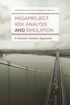
‘Technical risks’; ‘Economic risks’; ‘Environmental risks’ and ‘Political risks’ are other major parameters about whose level of impacts on the performance of the ETN project are uncertain. Figures A4–A7 show the comparative runs of these parameters.
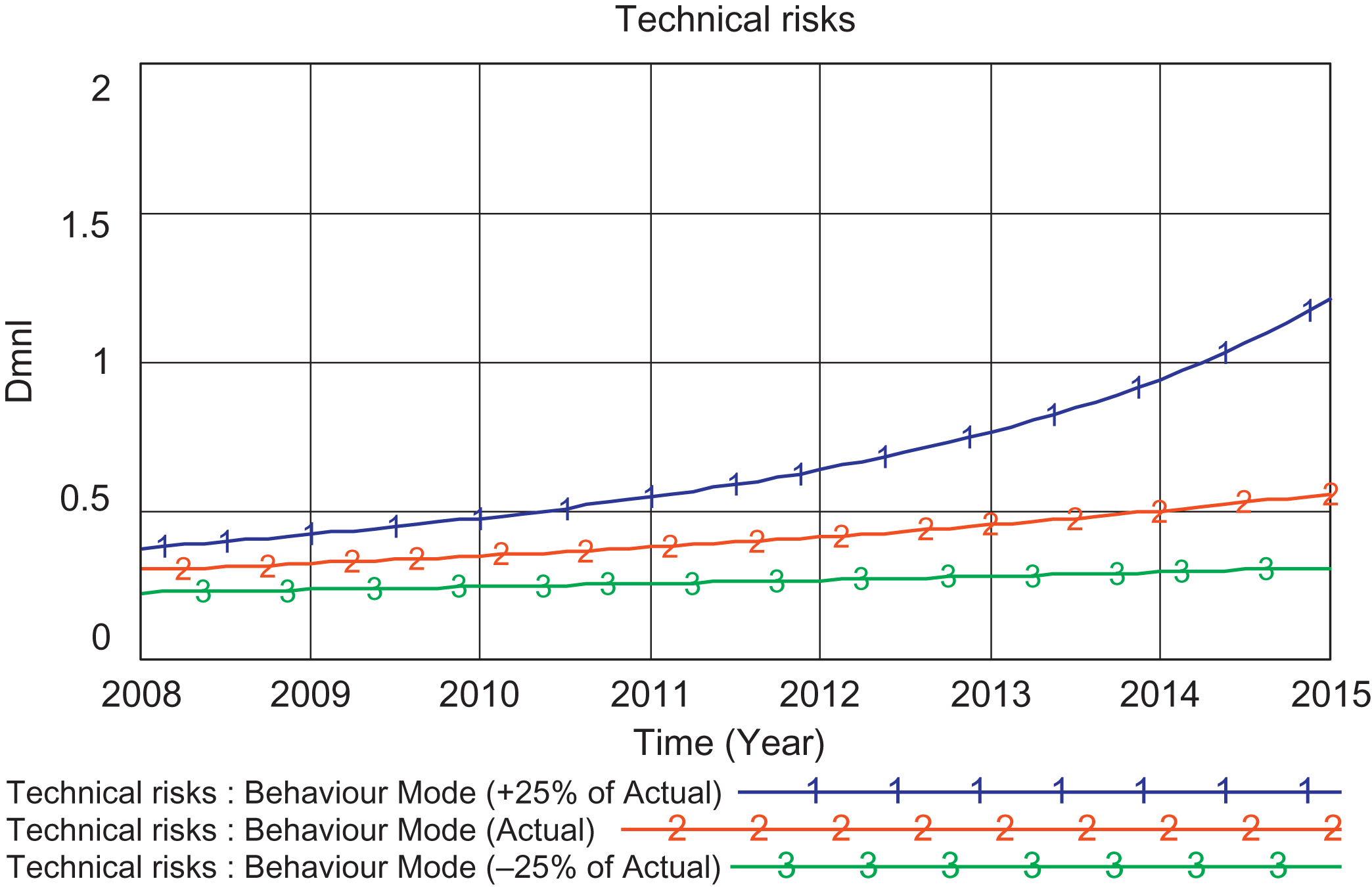


It is noticed again that although the behaviour modes of these risks look different from one another and from the social risks and social grievances, the general behaviours have not changed. Even when each of these risks starts out with a larger or smaller amount of parameter values, the behaviours of the stocks of the models will not change greatly.
As expected, changing the values of parameters in the model produces certain differences in the behaviours observed. Also, the sensitivity tests indicate that some parameter changes result in ‘greater’, or more significant, changes than others. For example, compare Figures A6 and A7. In Figure A6, the changes in ‘Environmental Issues from Works’ and ‘Unfavourable Climatic Conditions’ produce little difference in the behaviours, while in Figure A7, the curves show the same behaviours, but at different values of the stocks. This measure of more significant changes is studied through sensitivity analysis. In all cases, however, it is the structure of the system that primarily determines the behaviour mode. In general, but with exceptions, parameter values, when altered individually, only have a small influence on behaviour.
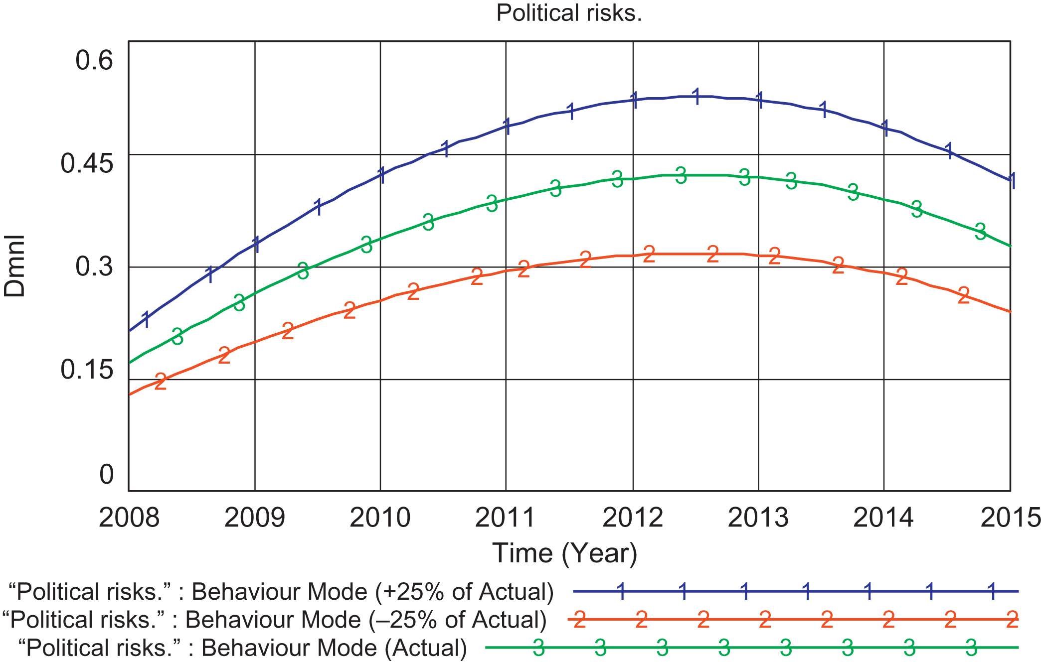
Now what should be expected if works on the ETN project are not completed as per the revised completion dates in summer 2014? That means there is a need for simulation to continue for another few months or even years. If so then will the uncertainties and risks continue to grow larger with time or not within the extended time? The situations represented in Figures A4–A7 are not the most likely outcomes. With a limited time available for works, one would expect the STEEP models to exhibit various shapes of growth over time. Monte Carlo simulation helps to generate most likely outcomes with dynamic confidence intervals for the trajectories of the variables in the STEEP models using the ranges of the probability distributions for the parameters represented in Table A3. The results of the Monte Carlo simulation are represented in Figures A8–A12. The figures show the 50%, 75%, 95% and 100% levels for social grievances, technical risks, economic risks, environmental risks and political risks in a sample of 500 simulations.

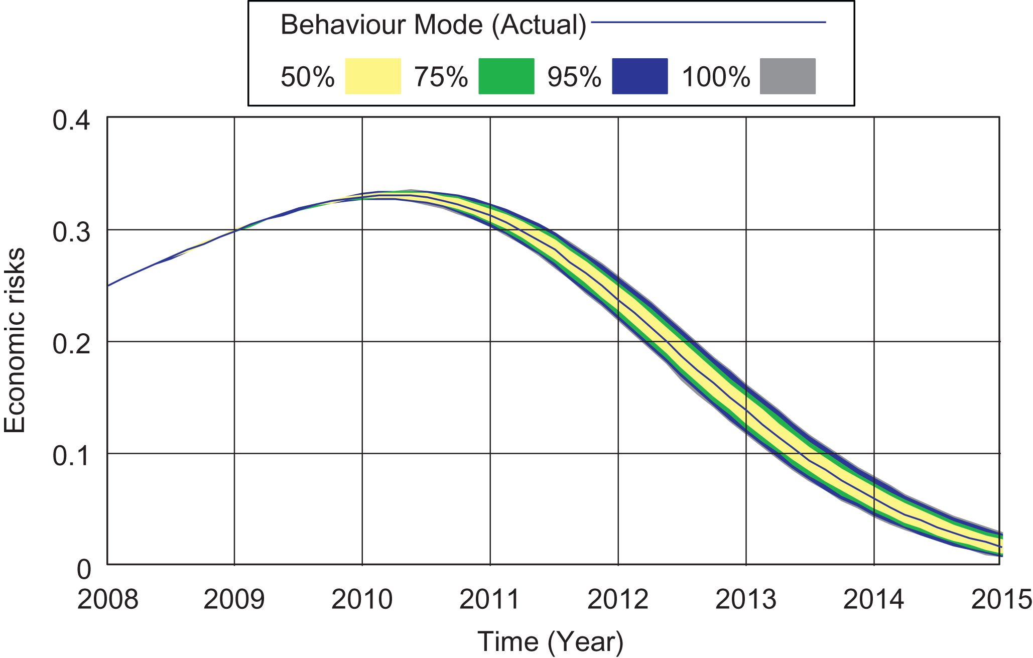

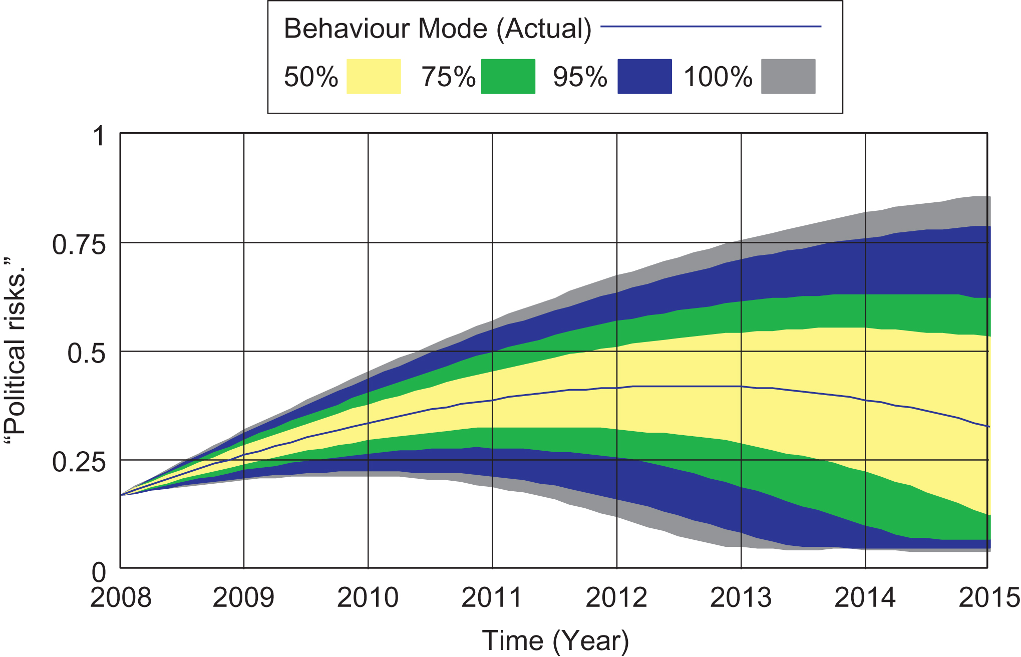
Figure A8 shows the sensitivity analysis of the social grievances. There are 0.06 (6%) of initial grievances level at the time of simulation, and the base case simulation (actual run) shows the grievance level growing to around 19% after two years. The confidence bounds show the same general pattern as in the actual base run. There is a narrow band of uncertainty in the first quarter of year 2008 when the project commenced but the width of the interval grows in an equilibrium form over time. By the year 2010, the 95% confidence bounds suggest that the level of social grievances as a result of the construction activities range from a low of 18% to as high as 22%. The eventual equilibrium is found when the positive and negative loops come into balance.
Similarly, in Figure A9, the analysis reveals that the width of the simulation intervals continue to grow larger over time. Narrow range of the technical risks in the early years of project development is typical to systems that are dominated by negative feedback loops. Differences in the input parameters are eventually overridden by the actions of the negative feedback loops and hence the technical uncertainties may shrink over time.
In the case of Figure A10, the narrowing in the range of economic risks between year 2008 and year 2010 seems similar to that of the technical risks but much more dominated by negative feedback loops in the systems. By the first quarter in year 2010, the width of the interval started to grow larger. However, the graph declines steadily over time. A similar result is seen in Figure A11.
Finally, Figure A12 shows a sensitivity analysis for the political risks model. The analysis reveals that the width of the simulation interval continues to grow larger over time. Until the 7th year (2015) of the simulation, there is a 50% chance that the level of political risks will be between 15% and 55%. By the same year, the 75% and the 95% confidence bounds suggest that the level of political risks could range from 10% to 65% and 5% to 80%, respectively.
A.9. Other Tests
The remainder of the tests under the model behaviour test, namely behaviour Anomaly; family member; surprise behaviour; extreme policy; behavioural boundary adequacy and statistical character are all interrelated, so the STEEP risk system models were tested concurrently with their respective questions indicated in Table A1 in mind. The main goal for these tests is to determine if the model responds as expected under abnormal conditions and if the model responds (or does not respond) when system variables of each sub model are changed from their baseline values. Therefore, tests for effects from extreme policies were performed on each model. During these tests, the integration system variables were the sole focus, since this is the focus of the research. Comparative traces of baseline, minimum and maximum values on each associated graph were also performed. Vensim software allows the modeller to simulate the same variable multiple times under differing conditions for each simulation run to allow comparison. Testing consisted of multiple simulation runs (and, as a result, multiple traces) of the same variable and graphed under different model conditions. Hence, each of the simulation runs and traces were represented by different behaviour based on the extreme points for the system variables being studied. In these cases, the variable scale was the same throughout each figure.
A.9.1. Policy Analysis, Design and Improvement
Once the model is fully tested and its properties understood, the final step is to test alternative new policies for system improvement. The system improvement tests ask whether the modelling process helps to change the system for better. To pass the test, the modelling process must identify policies that lead to improvement; those policies must be implemented for improved performance of the system. A policy is a decision rule, a general way of making decisions. In practice, assessing the impact of a model is extremely difficult. It is hard to assess the extent to which the modelling process will change people’s mental models and beliefs. It is rare for clients to adopt the recommendations of any model promptly or without modification.
In this last step, alternative policies are designed and tested by simulation runs to minimize risks at the construction phase of transportation megaprojects. It must be noted that many other variables and conditions may change at the same time the new policies are implemented, confounding attempts to attribute any results to the policies. Performance improvement following a study does not mean the model-based policies were responsible; the system may have improved for reasons unrelated to the modelling process. Likewise, deteriorating performance after policy implementation does not mean the models failed since the outcome could have been even worse without the new policies.
To improve the system, the policy analysis and design are performed by altering one or more characteristics of the STEEP models and examining the resulting behaviours. Like sensitivity analysis, policy analysis can also be numerical or pattern oriented. Pattern-oriented policy analysis is naturally much more important, since the purpose of system dynamics studies is to improve undesirable dynamic behaviour patterns. Policy design is determining what changes in the model structure and parameters would lead to improved model behaviour. While choosing the policies, practicality and usefulness have been checked with the experts and industrial stakeholders working on mega transportation projects.
With regard to the STEEP models, it is argued here that four central characteristics make these models well-suited for learning about and designing effective policies:
the feedback approach and emphasis on endogenous explanations of behaviour
the disaggregation approach
the simulation approach
the fact that the models are manageable enough such that their structures are clear and the links between structure and behaviour can be easily discovered through experimentation. Each of these four characteristics is explored in turn.
A.9.2. Feedback Approach
First, the STEEP models share feedback loop approaches to modelling endogenous sources of behaviour. The models illustrate how megaprojects under construction can be affected by risks and can endogenously create the conditions for time and cost overruns and quality deficiency once social, technical, economic, environmental and political uncertainties become high, causing excessive impact on project performance. By emphasizing feedback and an endogenous perspective, these system models will help policy-makers understand how policy resistance can arise. The models challenge common beliefs about how systems work by revealing feedback loops that can exacerbate the situation, thereby facilitating learning for even the most overconfident users.
A.9.3. Disaggregation Approach
Second, the MegaDS model takes a disaggregation approach to modelling. This implies that the STEEP system models are heterogeneous and do not track each individual model in the group, but instead are grouped in disaggregation. In keeping with the system dynamics modelling tradition, the building blocks of the model structure are stocks and flows rather than individual agents. However, these models are statistically estimated from data based on individual STEEP risk characteristics and level of impacts on a transportation megaproject. As such, a more efficient analysis, involving a better set of explanatory variables, can be carried out directly using disaggregated (i.e. individual risk level) data and model relationships. These reasons led to the development of the disaggregated models into five STEEP risk system models. The MegaDS model has five stocks each for the social, technical, economic and political sub models and four stocks for the environmental sub models (see Figure A13). All the models have common detailed implications of time and cost overruns and quality deficiency that arise from the interrelationship of variables within each sub system.

Figure A13
Disaggregation of the dynamic simulation models for transportation megaprojects. Note: The full figure can be found at: https://heriotwatt-my.sharepoint.com/personal/soo13_hw_ac_uk/_layouts/15/guestaccess.aspx?docid=0974bb3a6894a4271b31430b22fb7cac7&authkey=AZRBWHeTMYq4NSRcrwV4IJE
While there is much interest among modellers in an aggregated approach to the modelling of social problems, Rahmandad and Sterman (2008) argued that differential equation-based models — of which the models here are examples — are easier to understand and usually have similar policy implications when disaggregated. In addition, disaggregation reduces the models into manageable sizes, thereby decreasing the cost of developing and running complex models and allowing for easy but clear experimentation. Given limitations in individuals’ cognitive capacity, disaggregation also allows users to focus on feedback ahead of agent level detail and therefore develop a more holistic and endogenous perspective to the problem.
Further, recent research has shown that individuals often fail to understand the dynamics of accumulation (Sterman, 2008), with huge implications for the policies that they will then support. By focusing on stocks and flows as the building blocks of model structure, the STEEP models can directly help policy-makers build intuition regarding the dynamics of accumulation and thereby overcome one potential source of policy error.
A.9.4. Simulation Approach
Third, the reviewed models are running mathematical simulations that provide the opportunity to conduct experiments. While many lessons can be learned from a causal loop diagram, other more substantial insights require the development and testing of a simulation model. In both cases, simulation helps to illustrate why deliberate rational policies lead to policy resistance. In addition, the simulation models provide learning environments where modellers, policy-makers and other industrial stakeholders can design and test policies. Given the complexity of many policy environments, experimentation is essential for the design of effective policies. Simulations provide a helpful environment where policy-makers can experiment and learn about the effects of different policies without any significant social and economic cost for policy-makers.
Finally, simulations can help to build consensus surrounding difficult policy problems. By communicating the counter-intuitive nature of policy problems to policy-makers, simulations can encourage dialogue and lead to the development of shared interpretations regarding the source of problem behaviour. Even when different goals and value systems persist, simulation can help to focus the discussion on specific variables and outcomes that are the sources of divergence.
A.9.5. Manageable Model Size
Finally, the STEEP models are ‘manageable’. Here, we define ‘manageable’ to mean that the models consist of few significant stocks and feedback loops. There are two main benefits to these types of model sizes. First, they are small in size and allow for exhaustive experimentation through parameter changes. With these types of models, it is much easier to learn from sensitivity analysis (as shown in Figures A8–A12) and examine the interactions among different parameters. Thus, important leverage points in the system can more be easily identified.
Second, the manageable size ensures that the results of experiments can be fully and easily understood by policy-makers. Short exposition makes a holistic view possible. Due to the small size, individuals can see the feedback structure as a whole and not be frustrated by the need to track many variables and links at once. In addition, short exposition facilitates presentation of lessons to others, and helps bring the dynamic lessons to the meetings of stakeholders. Our emphasis on small models reflects that of Repenning (2003), who argues that in an academic context as well, small models are necessary to build the intuition of readers who are not accustomed to a dynamic or holistic view of systems.
In conclusion, manageable but small system dynamics models offer numerous benefits to the policy-making process during megaproject development. Table A9 summarizes the above discussion by depicting how each of the characteristics of the MegaDS models can help address the challenges inherent in policy-making during megaproject development.
The significance of the dynamics simulation models for transportation megaprojects in addressing policy problems.
| Policy problems characteristics | Model characteristics | |||
|---|---|---|---|---|
| Feedback approach | Disaggregated approach | Simulation approach | Manageable model size | |
| The policy resistance environment. | Feedback is the major source of policy resistance. | Accumulations (stocks) are essential to understanding policy resistance. | Simulation can illustrate why some intuitive policies lead to policy resistance and allow for the design and testing of more robust policies. | Small size allows for exhaustive experimentation and sensitivity analysis, wise interpretation of parameters and parameter changes. |
| Need to experiment and cost of experimenting. | Feedback diagrams and mental simulation models must substitute actual policy trials. | Disaggregate approach decreases the cost of developing and running complex models, allowing for more experimentation. | Simulations allow for exhaustive experimentation and games for policy-makers without incurring actual social and economic costs. | Small size ensures that the results of experiments can be fully and easily understood by policy-makers. |
| Need to persuade stakeholders. | Feedback diagrams and qualitative analysis can contribute to policy discussions. | Disaggregate approach facilitates presentation of lessons to others. Highlights feedback and endogenous sources of problem behaviour. | Simulations can help build consensus around difficult policy problems that may otherwise have multiple interpretations. | Small size facilitates presentation of lessons to others. Short exposition and holistic view made possible. |
| Overconfident policy-makers. | Causal loop (feedback) diagrams reveal new insights and challenge policy-makers to be wary of overconfidence. | Failure to understand the dynamics of accumulation is a common source of policy error. | Simulations effectively communicate the counter intuitive nature of policy problems to policy-makers who otherwise may remain not having been induced. | Small size ensures that model insights are fully understood, allowing policy-makers to appreciate and address their own overconfidence. |
| Need to have an endogenous perspective. | Feedback approach helps policy-makers learn what an endogenous view is and why it is necessary to effective policy-making. | Disaggregate approach creates room and flexibility in individuals’ cognitive capacity to concentrate on feedback and develop an endogenous perspective. | Simulations allow policy-makers to explore how behaviours are created endogenously through a broad model boundary. | Small size allows individuals to see the feedback structure as a whole and not be frustrated by the need to track many variables and links at once. |
Note: Project policy refers to principles, rules and guidelines formulated or adopted by an organization to reach its long-term goals and typically published in a booklet or other form that is widely accessible.
A.10. Policy Implementation
Having studied the influences of critical system variables on project performance for various simulation scenarios overtime, the megaproject managers can now implement appropriate policies that best suit the situation at hand to assess risks effectively. For best and worst case simulation scenarios that can inform project managers to design effective risk mitigation policies, the behaviour mode sensitivity graphs represented in Figures A3–A7 for the ETN project are typical examples.
Other recommendations to contractors involved in mega construction projects for policy implementation are:
Megaproject contractors must obtain assurances from the relevant government departments in the host country, especially as regards the availability of consents and permits.
The central bank of the host government may be persuaded to guarantee the availability of hard currency for export in connection with the project.
As a last resort, but an exercise which should be undertaken in any event, by a thorough review of the legal and regulatory regime in the country where the project is to be executed to ensure that all laws and regulations are strictly complied with and all the correct procedures are followed with a view to reducing the scope for challenges at a future date.
A.11. Summary
This penultimate section has addressed the validation of the model developed in this research. Unfortunately, there is no set of specific tests that can easily be applied to determine the ‘correctness’ of the MegaDS models. Furthermore, no algorithm exists to determine what techniques or procedures to use because every new simulation project presents a new and unique challenge.
In this study, two major groups of tests (empirical and rational) were carried out and described with and without field data. The empirical tests were conducted to examine the ability of the STEEP models to match the historical data of the ETN project. The findings of these tests from the simulated results on the level of risks impact on project cost and time and quality compared to the real system suggest that the models reflect reasonable predictive fit and could therefore be generalized.
On the other hand, the hypothesized system and the model system are used to conduct a series of rational tests, such as: parameter-verification, structure-verification, extreme policy tests and sensitivity tests. Throughout this process, the concepts, methodology and the findings of the research have been found to be reasonably supported by the extensive use of the Vensim software tools in support of the study. It is therefore contended that the developed model has the potential for subsequent development and use by practitioners.
Finally, it can be said that validation is both an art and a science, requiring creativity and insight. But validation is difficult to comprehend and has diverse procedures, and is unavoidable as it is the evidence for the steadfastness and legitimacy of the model. This chapter has provided an insight on the widely approved schemes of model validation and techniques in practice. The validation schemes can be applicable to quantitative (mathematical/computerized) as well as qualitative (conceptual) models. But reliability of the model can only be ascertained as the model passes more and more tests. Also, the decision of accepting a model as valid cannot be left to the modeller alone and inclusion of the industrial practitioners involved in megaprojects development in the validation procedure should be obligatory. Researchers and practitioners may find this chapter quite useful as the procedures for validation discussed are quite generic, and hence may be applied to other dynamic models as well. The next chapter therefore concludes the research by providing a summary of the work done, drawing the main conclusions arising from the study and making recommendations for future research.
Appendix B Structured Interview Questionnaire and Participants
Structured Interview Questionnaire
A Dynamic System Approach to Risk Assessment in Megaprojects
Profile/Demography of Interviewee
Type of Organisation: ________________ Date: __________ Time: _______
Type of Megaproject: ________________________________
Size of Megaproject: _______________________
Designation: ___________________
-
1.
Role/Responsibility of Interviewee
What was your role on the Project?
How long were you involved in mega construction projects?
-
2.
Project Goal/Scope
What were the main goals and objectives?
How did the project scope change over time?
-
3.
Generic Risk Events:
What were the generic risk events inherit in the project?
How did the generic risk events affect the project schedule overtime?
How did the generic risk events affect the project cost?
-
4.
Funding
Was the project funding source a dedicated fund source?
How were additional funds obtained as project costs increased?
Was the funding source stable over time?
- 5.
How can the qualitative risk effects on project performance be quantified and analyzed to reduce under performances in mega construction projects?
- 6.
How effective were the risks assessment practices used in managing/modelling risk interrelationships in megaprojects during construction?
Structured Interview Participants.
| No. | Company | Type of organization |
|---|---|---|
| 1 | Atkins | Consultant |
| 2 | Atkins PLC | Consultant |
| 3 | Bilfinger Berger/Siemens Consortium | Contractor |
| 4 | City of Edinburgh Council | Owner |
| 5 | Crummock (Scotland) Ltd. | Contractor |
| 6 | Farrans Construction | Contractor |
| 7 | Halcrow Group | Contractor |
| 8 | Jacobs Consultancy | Consultant |
| 9 | McNicholas Construction Co. Ltd | Contractor |
| 10 | Scottish Water | Consultant |
| 11 | Turner & Townsend | Consultant |
Appendix C Respondent’s Mean Scores of Importance
Respondent’s mean scores of importance for project objectives ( Po ).
| Considerations: cost, time and quality risks | |||||||||
|---|---|---|---|---|---|---|---|---|---|
| Number of respondents | Years of experience (Y) in % | Input (i) for cost (c), time (t) and quality (q) | Experimental input (Ei) Ei = Y × i | ||||||
| N | Yr. range | Year (Yr) | Y (%) | ic | it | iq | Y ic | Y it | Y iq |
| 1 | 11–20 | 16 | 1.1887 | 5 | 5 | 5 | 5.9435 | 5.9435 | 5.9435 |
| 2 | 11–20 | 16 | 1.1887 | 5 | 5 | 5 | 5.9435 | 5.9435 | 5.9435 |
| 3 | 11–20 | 16 | 1.1887 | 5 | 5 | 5 | 5.9435 | 5.9435 | 5.9435 |
| 4 | <5 | 5 | 0.3715 | 4 | 4 | 5 | 1.4859 | 1.4859 | 1.8574 |
| 5 | 11–20 | 16 | 1.1887 | 4 | 4 | 5 | 4.7548 | 4.7548 | 5.9435 |
| 6 | 0 | 0 | 0.0000 | 0 | 0 | 0 | 0.0000 | 0.0000 | 0.0000 |
| 7 | 21+ | 21 | 1.5602 | 4 | 4 | 4 | 6.2407 | 6.2407 | 6.2407 |
| 8 | 5–10 | 8 | 0.5944 | 0 | 0 | 0 | 0.0000 | 0.0000 | 0.0000 |
| 9 | 5–10 | 8 | 0.5944 | 3 | 5 | 3 | 1.7831 | 2.9718 | 1.7831 |
| 10 | 5–10 | 8 | 0.5944 | 3 | 3 | 3 | 1.7831 | 1.7831 | 1.7831 |
| 11 | 11–20 | 16 | 1.1887 | 5 | 4 | 5 | 5.9435 | 4.7548 | 5.9435 |
| 12 | 5–10 | 8 | 0.5944 | 0 | 0 | 0 | 0.0000 | 0.0000 | 0.0000 |
| 13 | 5–10 | 8 | 0.5944 | 5 | 2 | 3 | 2.9718 | 1.1887 | 1.7831 |
| 14 | 5–10 | 8 | 0.5944 | 4 | 1 | 5 | 2.3774 | 0.5944 | 2.9718 |
| 15 | 21+ | 21 | 1.5602 | 5 | 5 | 5 | 7.8009 | 7.8009 | 7.8009 |
| 16 | 11–20 | 16 | 1.1887 | 5 | 3 | 5 | 5.9435 | 3.5661 | 5.9435 |
| 17 | 0 | 0 | 0.0000 | 0 | 0 | 0 | 0.0000 | 0.0000 | 0.0000 |
| 18 | 21+ | 21 | 1.5602 | 0 | 0 | 0 | 0.0000 | 0.0000 | 0.0000 |
| 19 | 21+ | 21 | 1.5602 | 4 | 5 | 4 | 6.2407 | 7.8009 | 6.2407 |
| 20 | 11–20 | 16 | 1.1887 | 5 | 4 | 3 | 5.9435 | 4.7548 | 3.5661 |
| 21 | 11–20 | 16 | 1.1887 | 3 | 4 | 5 | 3.5661 | 4.7548 | 5.9435 |
| 22 | 5–10 | 8 | 0.5944 | 5 | 3 | 5 | 2.9718 | 1.7831 | 2.9718 |
| 23 | <5 | 5 | 0.3715 | 4 | 5 | 5 | 1.4859 | 1.8574 | 1.8574 |
| 24 | 5–10 | 8 | 0.5944 | 4 | 5 | 5 | 2.3774 | 2.9718 | 2.9718 |
| 25 | 5–10 | 8 | 0.5944 | 4 | 4 | 4 | 2.3774 | 2.3774 | 2.3774 |
| 26 | 5–10 | 8 | 0.5944 | 4 | 4 | 4 | 2.3774 | 2.3774 | 2.3774 |
| 27 | 5–10 | 8 | 0.5944 | 4 | 4 | 4 | 2.3774 | 2.3774 | 2.3774 |
| 28 | 11–20 | 16 | 1.1887 | 5 | 5 | 5 | 5.9435 | 5.9435 | 5.9435 |
| 29 | 21+ | 21 | 1.5602 | 5 | 5 | 5 | 7.8009 | 7.8009 | 7.8009 |
| 30 | 21+ | 21 | 1.5602 | 5 | 5 | 5 | 7.8009 | 7.8009 | 7.8009 |
| 31 | 5–10 | 8 | 0.5944 | 5 | 5 | 5 | 2.9718 | 2.9718 | 2.9718 |
| 32 | 5–10 | 8 | 0.5944 | 5 | 5 | 5 | 2.9718 | 2.9718 | 2.9718 |
| 33 | 5–10 | 8 | 0.5944 | 5 | 5 | 5 | 2.9718 | 2.9718 | 2.9718 |
| 34 | 5–10 | 8 | 0.5944 | 5 | 5 | 5 | 2.9718 | 2.9718 | 2.9718 |
| 35 | 5–10 | 8 | 0.5944 | 5 | 5 | 5 | 2.9718 | 2.9718 | 2.9718 |
| 36 | 11–20 | 16 | 1.1887 | 5 | 5 | 5 | 5.9435 | 5.9435 | 5.9435 |
| 37 | 21+ | 21 | 1.5602 | 5 | 5 | 5 | 7.8009 | 7.8009 | 7.8009 |
| 38 | 21+ | 21 | 1.5602 | 5 | 5 | 5 | 7.8009 | 7.8009 | 7.8009 |
| 39 | 21+ | 21 | 1.5602 | 5 | 5 | 5 | 7.8009 | 7.8009 | 7.8009 |
| 40 | 11–20 | 16 | 1.1887 | 5 | 5 | 5 | 5.9435 | 5.9435 | 5.9435 |
| 41 | 11–20 | 16 | 1.1887 | 5 | 5 | 5 | 5.9435 | 5.9435 | 5.9435 |
| 42 | 21+ | 21 | 1.5602 | 5 | 5 | 5 | 7.8009 | 7.8009 | 7.8009 |
| 43 | 11–20 | 16 | 1.1887 | 5 | 5 | 5 | 5.9435 | 5.9435 | 5.9435 |
| 44 | 21+ | 21 | 1.5602 | 0 | 0 | 0 | 0.0000 | 0.0000 | 0.0000 |
| 45 | 21+ | 21 | 1.5602 | 5 | 5 | 5 | 7.8009 | 7.8009 | 7.8009 |
| 46 | 11–20 | 16 | 1.1887 | 5 | 5 | 5 | 5.9435 | 5.9435 | 5.9435 |
| 47 | <5 | 5 | 0.3715 | 4 | 5 | 4 | 1.4859 | 1.8574 | 1.4859 |
| 48 | <5 | 5 | 0.3715 | 4 | 5 | 4 | 1.4859 | 1.8574 | 1.4859 |
| 49 | <5 | 5 | 0.3715 | 4 | 5 | 4 | 1.4859 | 1.8574 | 1.4859 |
| 50 | <5 | 5 | 0.3715 | 4 | 5 | 4 | 1.4859 | 1.8574 | 1.4859 |
| 51 | <5 | 5 | 0.3715 | 4 | 5 | 4 | 1.4859 | 1.8574 | 1.4859 |
| 52 | <5 | 5 | 0.3715 | 4 | 5 | 4 | 1.4859 | 1.8574 | 1.4859 |
| 53 | 11–20 | 16 | 1.1887 | 5 | 5 | 5 | 5.9435 | 5.9435 | 5.9435 |
| 54 | 11–20 | 16 | 1.1887 | 5 | 5 | 5 | 5.9435 | 5.9435 | 5.9435 |
| 55 | 21+ | 21 | 1.5602 | 5 | 5 | 5 | 7.8009 | 7.8009 | 7.8009 |
| 56 | 11–20 | 16 | 1.1887 | 5 | 5 | 5 | 5.9435 | 5.9435 | 5.9435 |
| 57 | 21+ | 21 | 1.5602 | 5 | 5 | 5 | 7.8009 | 7.8009 | 7.8009 |
| 58 | 21+ | 21 | 1.5602 | 5 | 5 | 5 | 7.8009 | 7.8009 | 7.8009 |
| 59 | 21+ | 21 | 1.5602 | 5 | 5 | 5 | 7.8009 | 7.8009 | 7.8009 |
| 60 | 21+ | 21 | 1.5602 | 5 | 5 | 5 | 7.8009 | 7.8009 | 7.8009 |
| 61 | 21+ | 21 | 1.5602 | 5 | 5 | 5 | 7.8009 | 7.8009 | 7.8009 |
| 62 | 21+ | 21 | 1.5602 | 5 | 5 | 5 | 7.8009 | 7.8009 | 7.8009 |
| 63 | 21+ | 21 | 1.5602 | 5 | 5 | 5 | 7.8009 | 7.8009 | 7.8009 |
| 64 | 21+ | 21 | 1.5602 | 5 | 5 | 5 | 7.8009 | 7.8009 | 7.8009 |
| 65 | 21+ | 21 | 1.5602 | 5 | 5 | 5 | 7.8009 | 7.8009 | 7.8009 |
| 66 | 21+ | 21 | 1.5602 | 5 | 5 | 5 | 7.8009 | 7.8009 | 7.8009 |
| 67 | 21+ | 21 | 1.5602 | 5 | 5 | 5 | 7.8009 | 7.8009 | 7.8009 |
| 68 | 21+ | 21 | 1.5602 | 5 | 5 | 5 | 7.8009 | 7.8009 | 7.8009 |
| 69 | 21+ | 21 | 1.5602 | 5 | 5 | 5 | 7.8009 | 7.8009 | 7.8009 |
| 70 | 11–20 | 16 | 1.1887 | 5 | 5 | 5 | 5.9435 | 5.9435 | 5.9435 |
| 71 | 21+ | 21 | 1.5602 | 5 | 5 | 5 | 7.8009 | 7.8009 | 7.8009 |
| 72 | 5–10 | 8 | 0.5944 | 5 | 5 | 5 | 2.9718 | 2.9718 | 2.9718 |
| 73 | 5–10 | 8 | 0.5944 | 5 | 5 | 5 | 2.9718 | 2.9718 | 2.9718 |
| 74 | 11–20 | 16 | 1.1887 | 5 | 5 | 5 | 5.9435 | 5.9435 | 5.9435 |
| 75 | 21+ | 21 | 1.5602 | 4 | 4 | 3 | 6.2407 | 6.2407 | 4.6805 |
| 76 | 21+ | 21 | 1.5602 | 4 | 4 | 5 | 6.2407 | 6.2407 | 7.8009 |
| 77 | 21+ | 21 | 1.5602 | 4 | 4 | 5 | 6.2407 | 6.2407 | 7.8009 |
| 78 | 11–20 | 16 | 1.1887 | 4 | 4 | 4 | 4.7548 | 4.7548 | 4.7548 |
| 79 | 11–20 | 16 | 1.1887 | 4 | 4 | 4 | 4.7548 | 4.7548 | 4.7548 |
| 80 | 21+ | 21 | 1.5602 | 3 | 5 | 3 | 4.6805 | 7.8009 | 4.6805 |
| 81 | 11–20 | 16 | 1.1887 | 3 | 3 | 3 | 3.5661 | 3.5661 | 3.5661 |
| 82 | 21+ | 21 | 1.5602 | 5 | 4 | 5 | 7.8009 | 6.2407 | 7.8009 |
| 83 | 21+ | 21 | 1.5602 | 4 | 4 | 5 | 6.2407 | 6.2407 | 7.8009 |
| 84 | 11–20 | 16 | 1.1887 | 5 | 2 | 3 | 5.9435 | 2.3774 | 3.5661 |
| 85 | 11–20 | 16 | 1.1887 | 4 | 1 | 5 | 4.7548 | 1.1887 | 5.9435 |
| 86 | 11–20 | 16 | 1.1887 | 5 | 5 | 5 | 5.9435 | 5.9435 | 5.9435 |
| 87 | 21+ | 21 | 1.5602 | 5 | 3 | 5 | 7.8009 | 4.6805 | 7.8009 |
| 88 | 11–20 | 16 | 1.1887 | 4 | 3 | 5 | 4.7548 | 3.5661 | 5.9435 |
| 89 | 11–20 | 16 | 1.1887 | 4 | 3 | 5 | 4.7548 | 3.5661 | 5.9435 |
| 90 | 11–20 | 16 | 1.1887 | 4 | 5 | 4 | 4.7548 | 5.9435 | 4.7548 |
| Total | 1,346 | 100.0000 | 444.58 | 432.32 | 450.8 | ||||
| Mean value (MVpo) | = | |∑EiX1–3|/Ntotal | 4.9 | 4.8 | 5.0 | ||||
Notes: Ei, experimental input; X, value for individual experimental inputs for cost, time and quality; i, respondents inputs; X1 = ic = respondents inputs for project cost; X2 = it = respondents inputs for project time; X3 = iq = respondents inputs for project quality; Ntotal, total number of respondents.
Respondent’s mean scores of importance for potential risks (PR1): Social risks.
| Number of respondents | Years of experience (Y) in % | Input (i) for G1 under cost (c), time (t) and quality (q) | Experimental input (Ei) Ei = Y × i | ||||||
|---|---|---|---|---|---|---|---|---|---|
| N | Yr. Range | Year (Yr) | Y (%) | ic | it | Iq | Y ic | Y it | Y iq |
| 1 | 11–20 | 16 | 1.1887 | 4 | 5 | 2 | 4.7548 | 5.9435 | 2.3774 |
| 2 | 11–20 | 16 | 1.1887 | 4 | 5 | 2 | 4.7548 | 5.9435 | 2.3774 |
| 3 | 11–20 | 16 | 1.1887 | 5 | 5 | 5 | 5.9435 | 5.9435 | 5.9435 |
| 4 | <5 | 5 | 0.3715 | 3 | 1 | 3 | 1.1144 | 0.3715 | 1.1144 |
| 5 | 11–20 | 16 | 1.1887 | 4 | 3 | 4 | 4.7548 | 3.5661 | 4.7548 |
| 6 | 0 | 0 | 0.0000 | 0 | 0 | 0 | 0.0000 | 0.0000 | 0.0000 |
| 7 | 21+ | 21 | 1.5602 | 3 | 3 | 3 | 4.6805 | 4.6805 | 4.6805 |
| 8 | 5–10 | 8 | 0.5944 | 0 | 0 | 0 | 0.0000 | 0.0000 | 0.0000 |
| 9 | 5–10 | 8 | 0.5944 | 2 | 4 | 3 | 1.1887 | 2.3774 | 1.7831 |
| 10 | 5–10 | 8 | 0.5944 | 2 | 3 | 3 | 1.1887 | 1.7831 | 1.7831 |
| 11 | 11–20 | 16 | 1.1887 | 5 | 5 | 5 | 5.9435 | 5.9435 | 5.9435 |
| 12 | 5–10 | 8 | 0.5944 | 0 | 0 | 0 | 0.0000 | 0.0000 | 0.0000 |
| 13 | 5–10 | 8 | 0.5944 | 0 | 0 | 0 | 0.0000 | 0.0000 | 0.0000 |
| 14 | 5–10 | 8 | 0.5944 | 0 | 0 | 0 | 0.0000 | 0.0000 | 0.0000 |
| 15 | 21+ | 21 | 1.5602 | 5 | 5 | 2 | 7.8009 | 7.8009 | 3.1204 |
| 16 | 11–20 | 16 | 1.1887 | 5 | 5 | 3 | 5.9435 | 5.9435 | 3.5661 |
| 17 | 0 | 0 | 0.0000 | 0 | 0 | 0 | 0.0000 | 0.0000 | 0.0000 |
| 18 | 21+ | 21 | 1.5602 | 0 | 0 | 0 | 0.0000 | 0.0000 | 0.0000 |
| 19 | 21+ | 21 | 1.5602 | 0 | 0 | 0 | 0.0000 | 0.0000 | 0.0000 |
| 20 | 11–20 | 16 | 1.1887 | 4 | 5 | 4 | 4.7548 | 5.9435 | 4.7548 |
| 21 | 11–20 | 16 | 1.1887 | 0 | 0 | 0 | 0.0000 | 0.0000 | 0.0000 |
| 22 | 5–10 | 8 | 0.5944 | 4 | 5 | 5 | 2.3774 | 2.9718 | 2.9718 |
| 23 | <5 | 5 | 0.3715 | 0 | 0 | 0 | 0.0000 | 0.0000 | 0.0000 |
| 24 | 5–10 | 8 | 0.5944 | 5 | 3 | 1 | 2.9718 | 1.7831 | 0.5944 |
| 25 | 5–10 | 8 | 0.5944 | 5 | 3 | 1 | 2.9718 | 1.7831 | 0.5944 |
| 26 | 5–10 | 8 | 0.5944 | 5 | 3 | 1 | 2.9718 | 1.7831 | 0.5944 |
| 27 | 5–10 | 8 | 0.5944 | 5 | 3 | 1 | 2.9718 | 1.7831 | 0.5944 |
| 28 | 11–20 | 16 | 1.1887 | 5 | 5 | 5 | 5.9435 | 5.9435 | 5.9435 |
| 29 | 21+ | 21 | 1.5602 | 2 | 2 | 2 | 3.1204 | 3.1204 | 3.1204 |
| 30 | 21+ | 21 | 1.5602 | 4 | 4 | 4 | 6.2407 | 6.2407 | 6.2407 |
| 31 | 5–10 | 8 | 0.5944 | 5 | 4 | 1 | 2.9718 | 2.3774 | 0.5944 |
| 32 | 5–10 | 8 | 0.5944 | 5 | 4 | 1 | 2.9718 | 2.3774 | 0.5944 |
| 33 | 5–10 | 8 | 0.5944 | 5 | 4 | 1 | 2.9718 | 2.3774 | 0.5944 |
| 34 | 5–10 | 8 | 0.5944 | 5 | 4 | 1 | 2.9718 | 2.3774 | 0.5944 |
| 35 | 5–10 | 8 | 0.5944 | 5 | 4 | 1 | 2.9718 | 2.3774 | 0.5944 |
| 36 | 11–20 | 16 | 1.1887 | 2 | 4 | 1 | 2.3774 | 4.7548 | 1.1887 |
| 37 | 21+ | 21 | 1.5602 | 4 | 4 | 1 | 6.2407 | 6.2407 | 1.5602 |
| 38 | 21+ | 21 | 1.5602 | 5 | 5 | 5 | 7.8009 | 7.8009 | 7.8009 |
| 39 | 21+ | 21 | 1.5602 | 0 | 0 | 0 | 0.0000 | 0.0000 | 0.0000 |
| 40 | 11–20 | 16 | 1.1887 | 0 | 0 | 0 | 0.0000 | 0.0000 | 0.0000 |
| 41 | 11–20 | 16 | 1.1887 | 5 | 5 | 5 | 5.9435 | 5.9435 | 5.9435 |
| 42 | 21+ | 21 | 1.5602 | 0 | 0 | 0 | 0.0000 | 0.0000 | 0.0000 |
| 43 | 11–20 | 16 | 1.1887 | 5 | 5 | 5 | 5.9435 | 5.9435 | 5.9435 |
| 44 | 21+ | 21 | 1.5602 | 0 | 0 | 0 | 0.0000 | 0.0000 | 0.0000 |
| 45 | 21+ | 21 | 1.5602 | 5 | 5 | 5 | 7.8009 | 7.8009 | 7.8009 |
| 46 | 11–20 | 16 | 1.1887 | 0 | 0 | 0 | 0.0000 | 0.0000 | 0.0000 |
| 47 | < 5 | 5 | 0.3715 | 5 | 2 | 2 | 1.8574 | 0.7429 | 0.7429 |
| 48 | <5 | 5 | 0.3715 | 5 | 2 | 2 | 1.8574 | 0.7429 | 0.7429 |
| 49 | <5 | 5 | 0.3715 | 3 | 2 | 2 | 1.1144 | 0.7429 | 0.7429 |
| 50 | <5 | 5 | 0.3715 | 5 | 2 | 2 | 1.8574 | 0.7429 | 0.7429 |
| 51 | <5 | 5 | 0.3715 | 5 | 2 | 2 | 1.8574 | 0.7429 | 0.7429 |
| 52 | <5 | 5 | 0.3715 | 3 | 2 | 2 | 1.1144 | 0.7429 | 0.7429 |
| 53 | 11–20 | 16 | 1.1887 | 0 | 0 | 0 | 0.0000 | 0.0000 | 0.0000 |
| 54 | 11–20 | 16 | 1.1887 | 0 | 0 | 0 | 0.0000 | 0.0000 | 0.0000 |
| 55 | 21+ | 21 | 1.5602 | 5 | 4 | 3 | 7.8009 | 6.2407 | 4.6805 |
| 56 | 11–20 | 16 | 1.1887 | 5 | 4 | 3 | 5.9435 | 4.7548 | 3.5661 |
| 57 | 21+ | 21 | 1.5602 | 5 | 5 | 3 | 7.8009 | 7.8009 | 4.6805 |
| 58 | 21+ | 21 | 1.5602 | 5 | 4 | 3 | 7.8009 | 6.2407 | 4.6805 |
| 59 | 21+ | 21 | 1.5602 | 5 | 4 | 1 | 7.8009 | 6.2407 | 1.5602 |
| 60 | 21+ | 21 | 1.5602 | 5 | 4 | 3 | 7.8009 | 6.2407 | 4.6805 |
| 61 | 21+ | 21 | 1.5602 | 5 | 4 | 1 | 7.8009 | 6.2407 | 1.5602 |
| 62 | 21+ | 21 | 1.5602 | 5 | 4 | 3 | 7.8009 | 6.2407 | 4.6805 |
| 63 | 21+ | 21 | 1.5602 | 5 | 5 | 2 | 7.8009 | 7.8009 | 3.1204 |
| 64 | 21+ | 21 | 1.5602 | 5 | 5 | 2 | 7.8009 | 7.8009 | 3.1204 |
| 65 | 21+ | 21 | 1.5602 | 5 | 5 | 1 | 7.8009 | 7.8009 | 1.5602 |
| 66 | 21+ | 21 | 1.5602 | 5 | 5 | 2 | 7.8009 | 7.8009 | 3.1204 |
| 67 | 21+ | 21 | 1.5602 | 5 | 4 | 1 | 7.8009 | 6.2407 | 1.5602 |
| 68 | 21+ | 21 | 1.5602 | 5 | 4 | 5 | 7.8009 | 6.2407 | 7.8009 |
| 69 | 21+ | 21 | 1.5602 | 5 | 5 | 4 | 7.8009 | 7.8009 | 6.2407 |
| 70 | 11–20 | 16 | 1.1887 | 5 | 4 | 4 | 5.9435 | 4.7548 | 4.7548 |
| 71 | 21+ | 21 | 1.5602 | 5 | 5 | 5 | 7.8009 | 7.8009 | 7.8009 |
| 72 | 5–10 | 8 | 0.5944 | 4 | 5 | 4 | 2.3774 | 2.9718 | 2.3774 |
| 73 | 5–10 | 8 | 0.5944 | 5 | 5 | 3 | 2.9718 | 2.9718 | 1.7831 |
| 74 | 11–20 | 16 | 1.1887 | 2 | 2 | 1 | 2.3774 | 2.3774 | 1.1887 |
| 75 | 21+ | 21 | 1.5602 | 5 | 2 | 2 | 7.8009 | 3.1204 | 3.1204 |
| 76 | 21+ | 21 | 1.5602 | 5 | 2 | 2 | 7.8009 | 3.1204 | 3.1204 |
| 77 | 21+ | 21 | 1.5602 | 2 | 2 | 2 | 3.1204 | 3.1204 | 3.1204 |
| 78 | 11–20 | 16 | 1.1887 | 1 | 1 | 1 | 1.1887 | 1.1887 | 1.1887 |
| 79 | 11–20 | 16 | 1.1887 | 3 | 4 | 3 | 3.5661 | 4.7548 | 3.5661 |
| 80 | 21+ | 21 | 1.5602 | 5 | 3 | 1 | 7.8009 | 4.6805 | 1.5602 |
| 81 | 11–20 | 16 | 1.1887 | 5 | 3 | 1 | 5.9435 | 3.5661 | 1.1887 |
| 82 | 21+ | 21 | 1.5602 | 5 | 3 | 1 | 7.8009 | 4.6805 | 1.5602 |
| 83 | 21+ | 21 | 1.5602 | 5 | 4 | 1 | 7.8009 | 6.2407 | 1.5602 |
| 84 | 11–20 | 16 | 1.1887 | 5 | 4 | 3 | 5.9435 | 4.7548 | 3.5661 |
| 85 | 11–20 | 16 | 1.1887 | 5 | 3 | 2 | 5.9435 | 3.5661 | 2.3774 |
| 86 | 11–20 | 16 | 1.1887 | 5 | 3 | 3 | 5.9435 | 3.5661 | 3.5661 |
| 87 | 21+ | 21 | 1.5602 | 5 | 3 | 2 | 7.8009 | 4.6805 | 3.1204 |
| 88 | 11–20 | 16 | 1.1887 | 5 | 4 | 2 | 5.9435 | 4.7548 | 2.3774 |
| 89 | 11–20 | 16 | 1.1887 | 5 | 3 | 3 | 5.9435 | 3.5661 | 3.5661 |
| 90 | 11–20 | 16 | 1.1887 | 5 | 3 | 2 | 5.9435 | 3.5661 | 2.3774 |
| Total | 1346 | 100.00 | 375.93 | 321.77 | 215.97 | ||||
| Mean value (MVPR1) | = | |∑EiX1–3|/Ntotal | 4.2 | 3.6 | 2.4 | ||||
Notes: Ei, experimental input; X, value for individual experimental inputs for cost, time and quality; i, respondents inputs; X1 = ic = respondents inputs for project cost; X2 = it = respondents inputs for project time; X3 = iq = respondents inputs for project quality; Ntotal = total number of respondents.
Respondent’s mean scores of importance for potential risks (PR2): Technical risks.
| Number of respondents | Years of experience (Y) in % | Input (i) for G2 under cost (c), time (t) and quality (q) | Experimental input (Ei) Ei = Y × i | ||||||
|---|---|---|---|---|---|---|---|---|---|
| N | Yr. range | Year (Yr) | Y (%) | ic | it | iq | Y ic | Y it | Y iq |
| 1 | 11–20 | 16 | 1.1887 | 5 | 5 | 5 | 5.9435 | 5.9435 | 5.9435 |
| 2 | 11–20 | 16 | 1.1887 | 5 | 5 | 5 | 5.9435 | 5.9435 | 5.9435 |
| 3 | 11–20 | 16 | 1.1887 | 5 | 5 | 5 | 5.9435 | 5.9435 | 5.9435 |
| 4 | <5 | 5 | 0.3715 | 3 | 4 | 3 | 1.1144 | 1.4859 | 1.1144 |
| 5 | 11–20 | 16 | 1.1887 | 3 | 3 | 3 | 3.5661 | 3.5661 | 3.5661 |
| 6 | 0 | 0 | 0.0000 | 0 | 0 | 0 | 0.0000 | 0.0000 | 0.0000 |
| 7 | 21+ | 21 | 1.5602 | 3 | 3 | 3 | 4.6805 | 4.6805 | 4.6805 |
| 8 | 5–10 | 8 | 0.5944 | 0 | 0 | 0 | 0.0000 | 0.0000 | 0.0000 |
| 9 | 5–10 | 8 | 0.5944 | 3 | 3 | 3 | 1.7831 | 1.7831 | 1.7831 |
| 10 | 5–10 | 8 | 0.5944 | 3 | 2 | 2 | 1.7831 | 1.1887 | 1.1887 |
| 11 | 11–20 | 16 | 1.1887 | 5 | 5 | 5 | 5.9435 | 5.9435 | 5.9435 |
| 12 | 5–10 | 8 | 0.5944 | 5 | 5 | 5 | 2.9718 | 2.9718 | 2.9718 |
| 13 | 5–10 | 8 | 0.5944 | 5 | 5 | 5 | 2.9718 | 2.9718 | 2.9718 |
| 14 | 5–10 | 8 | 0.5944 | 5 | 5 | 5 | 2.9718 | 2.9718 | 2.9718 |
| 15 | 21+ | 21 | 1.5602 | 5 | 5 | 5 | 7.8009 | 7.8009 | 7.8009 |
| 16 | 11–20 | 16 | 1.1887 | 5 | 5 | 4 | 5.9435 | 5.9435 | 4.7548 |
| 17 | 0 | 0 | 0.0000 | 0 | 0 | 0 | 0.0000 | 0.0000 | 0.0000 |
| 18 | 21+ | 21 | 1.5602 | 0 | 0 | 0 | 0.0000 | 0.0000 | 0.0000 |
| 19 | 21+ | 21 | 1.5602 | 0 | 0 | 0 | 0.0000 | 0.0000 | 0.0000 |
| 20 | 11–20 | 16 | 1.1887 | 4 | 4 | 4 | 4.7548 | 4.7548 | 4.7548 |
| 21 | 11–20 | 16 | 1.1887 | 3 | 2 | 5 | 3.5661 | 2.3774 | 5.9435 |
| 22 | 5–10 | 8 | 0.5944 | 4 | 4 | 4 | 2.3774 | 2.3774 | 2.3774 |
| 23 | <5 | 5 | 0.3715 | 5 | 5 | 4 | 1.8574 | 1.8574 | 1.4859 |
| 24 | 5–10 | 8 | 0.5944 | 5 | 5 | 5 | 2.9718 | 2.9718 | 2.9718 |
| 25 | 5–10 | 8 | 0.5944 | 4 | 4 | 4 | 2.3774 | 2.3774 | 2.3774 |
| 26 | 5–10 | 8 | 0.5944 | 4 | 4 | 4 | 2.3774 | 2.3774 | 2.3774 |
| 27 | 5–10 | 8 | 0.5944 | 4 | 4 | 4 | 2.3774 | 2.3774 | 2.3774 |
| 28 | 11–20 | 16 | 1.1887 | 4 | 4 | 5 | 4.7548 | 4.7548 | 5.9435 |
| 29 | 21+ | 21 | 1.5602 | 1 | 2 | 1 | 1.5602 | 3.1204 | 1.5602 |
| 30 | 21+ | 21 | 1.5602 | 4 | 4 | 4 | 6.2407 | 6.2407 | 6.2407 |
| 31 | 5–10 | 8 | 0.5944 | 5 | 5 | 5 | 2.9718 | 2.9718 | 2.9718 |
| 32 | 5–10 | 8 | 0.5944 | 5 | 5 | 5 | 2.9718 | 2.9718 | 2.9718 |
| 33 | 5–10 | 8 | 0.5944 | 5 | 5 | 5 | 2.9718 | 2.9718 | 2.9718 |
| 34 | 5–10 | 8 | 0.5944 | 5 | 5 | 5 | 2.9718 | 2.9718 | 2.9718 |
| 35 | 5–10 | 8 | 0.5944 | 5 | 5 | 5 | 2.9718 | 2.9718 | 2.9718 |
| 36 | 11–20 | 16 | 1.1887 | 4 | 4 | 2 | 4.7548 | 4.7548 | 2.3774 |
| 37 | 21+ | 21 | 1.5602 | 5 | 5 | 5 | 7.8009 | 7.8009 | 7.8009 |
| 38 | 21+ | 21 | 1.5602 | 5 | 5 | 4 | 7.8009 | 7.8009 | 6.2407 |
| 39 | 21+ | 21 | 1.5602 | 5 | 5 | 5 | 7.8009 | 7.8009 | 7.8009 |
| 40 | 11–20 | 16 | 1.1887 | 5 | 5 | 5 | 5.9435 | 5.9435 | 5.9435 |
| 41 | 11–20 | 16 | 1.1887 | 5 | 5 | 5 | 5.9435 | 5.9435 | 5.9435 |
| 42 | 21+ | 21 | 1.5602 | 5 | 5 | 5 | 7.8009 | 7.8009 | 7.8009 |
| 43 | 11–20 | 16 | 1.1887 | 5 | 5 | 5 | 5.9435 | 5.9435 | 5.9435 |
| 44 | 21+ | 21 | 1.5602 | 0 | 0 | 0 | 0.0000 | 0.0000 | 0.0000 |
| 45 | 21+ | 21 | 1.5602 | 5 | 5 | 5 | 7.8009 | 7.8009 | 7.8009 |
| 46 | 11–20 | 16 | 1.1887 | 5 | 5 | 5 | 5.9435 | 5.9435 | 5.9435 |
| 47 | <5 | 5 | 0.3715 | 2 | 3 | 2 | 0.7429 | 1.1144 | 0.7429 |
| 48 | <5 | 5 | 0.3715 | 2 | 3 | 2 | 0.7429 | 1.1144 | 0.7429 |
| 49 | <5 | 5 | 0.3715 | 2 | 3 | 2 | 0.7429 | 1.1144 | 0.7429 |
| 50 | <5 | 5 | 0.3715 | 2 | 3 | 2 | 0.7429 | 1.1144 | 0.7429 |
| 51 | <5 | 5 | 0.3715 | 2 | 3 | 2 | 0.7429 | 1.1144 | 0.7429 |
| 52 | <5 | 5 | 0.3715 | 2 | 3 | 2 | 0.7429 | 1.1144 | 0.7429 |
| 53 | 11–20 | 16 | 1.1887 | 5 | 5 | 5 | 5.9435 | 5.9435 | 5.9435 |
| 54 | 11–20 | 16 | 1.1887 | 5 | 5 | 5 | 5.9435 | 5.9435 | 5.9435 |
| 55 | 21+ | 21 | 1.5602 | 5 | 5 | 5 | 7.8009 | 7.8009 | 7.8009 |
| 56 | 11–20 | 16 | 1.1887 | 5 | 5 | 5 | 5.9435 | 5.9435 | 5.9435 |
| 57 | 21+ | 21 | 1.5602 | 5 | 5 | 5 | 7.8009 | 7.8009 | 7.8009 |
| 58 | 21+ | 21 | 1.5602 | 5 | 5 | 5 | 7.8009 | 7.8009 | 7.8009 |
| 59 | 21+ | 21 | 1.5602 | 5 | 5 | 5 | 7.8009 | 7.8009 | 7.8009 |
| 60 | 21+ | 21 | 1.5602 | 5 | 5 | 5 | 7.8009 | 7.8009 | 7.8009 |
| 61 | 21+ | 21 | 1.5602 | 5 | 5 | 5 | 7.8009 | 7.8009 | 7.8009 |
| 62 | 21+ | 21 | 1.5602 | 5 | 5 | 5 | 7.8009 | 7.8009 | 7.8009 |
| 63 | 21+ | 21 | 1.5602 | 5 | 5 | 5 | 7.8009 | 7.8009 | 7.8009 |
| 64 | 21+ | 21 | 1.5602 | 5 | 5 | 5 | 7.8009 | 7.8009 | 7.8009 |
| 65 | 21+ | 21 | 1.5602 | 5 | 5 | 5 | 7.8009 | 7.8009 | 7.8009 |
| 66 | 21+ | 21 | 1.5602 | 5 | 5 | 5 | 7.8009 | 7.8009 | 7.8009 |
| 67 | 21+ | 21 | 1.5602 | 5 | 5 | 5 | 7.8009 | 7.8009 | 7.8009 |
| 68 | 21+ | 21 | 1.5602 | 5 | 5 | 5 | 7.8009 | 7.8009 | 7.8009 |
| 69 | 21+ | 21 | 1.5602 | 5 | 5 | 5 | 7.8009 | 7.8009 | 7.8009 |
| 70 | 11–20 | 16 | 1.1887 | 5 | 5 | 5 | 5.9435 | 5.9435 | 5.9435 |
| 71 | 21+ | 21 | 1.5602 | 5 | 5 | 5 | 7.8009 | 7.8009 | 7.8009 |
| 72 | 5–10 | 8 | 0.5944 | 5 | 5 | 5 | 2.9718 | 2.9718 | 2.9718 |
| 73 | 5–10 | 8 | 0.5944 | 5 | 5 | 5 | 2.9718 | 2.9718 | 2.9718 |
| 74 | 11–20 | 16 | 1.1887 | 3 | 4 | 3 | 3.5661 | 4.7548 | 3.5661 |
| 75 | 21+ | 21 | 1.5602 | 3 | 3 | 3 | 4.6805 | 4.6805 | 4.6805 |
| 76 | 21+ | 21 | 1.5602 | 3 | 3 | 3 | 4.6805 | 4.6805 | 4.6805 |
| 77 | 21+ | 21 | 1.5602 | 3 | 3 | 3 | 4.6805 | 4.6805 | 4.6805 |
| 78 | 11–20 | 16 | 1.1887 | 3 | 3 | 3 | 3.5661 | 3.5661 | 3.5661 |
| 79 | 11–20 | 16 | 1.1887 | 3 | 3 | 3 | 3.5661 | 3.5661 | 3.5661 |
| 80 | 21+ | 21 | 1.5602 | 3 | 2 | 2 | 4.6805 | 3.1204 | 3.1204 |
| 81 | 11–20 | 16 | 1.1887 | 5 | 5 | 5 | 5.9435 | 5.9435 | 5.9435 |
| 82 | 21+ | 21 | 1.5602 | 5 | 5 | 5 | 7.8009 | 7.8009 | 7.8009 |
| 83 | 21+ | 21 | 1.5602 | 5 | 5 | 5 | 7.8009 | 7.8009 | 7.8009 |
| 84 | 11–20 | 16 | 1.1887 | 5 | 5 | 5 | 5.9435 | 5.9435 | 5.9435 |
| 85 | 11–20 | 16 | 1.1887 | 5 | 5 | 5 | 5.9435 | 5.9435 | 5.9435 |
| 86 | 11–20 | 16 | 1.1887 | 5 | 5 | 4 | 5.9435 | 5.9435 | 4.7548 |
| 87 | 21+ | 21 | 1.5602 | 5 | 5 | 4 | 7.8009 | 7.8009 | 6.2407 |
| 88 | 11–20 | 16 | 1.1887 | 5 | 5 | 4 | 5.9435 | 5.9435 | 4.7548 |
| 89 | 11–20 | 16 | 1.1887 | 5 | 5 | 4 | 5.9435 | 5.9435 | 4.7548 |
| 90 | 11–20 | 16 | 1.1887 | 5 | 5 | 4 | 5.9435 | 5.9435 | 4.7548 |
| Total | 1346 | 100.00 | 422.59 | 424.59 | 412.18 | ||||
| Mean value (MVPR2) | = | |∑EiX1–3|/Ntotal | 4.7 | 4.7 | 4.6 | ||||
Notes: Ei, experimental input; X, value for individual experimental inputs for cost, time and quality, i, respondents inputs, X1 = ic = respondents inputs for project cost, X2 = it = respondents inputs for project time; X3 = iq = respondents inputs for project quality; Ntotal, total number of respondents.
Respondent’s mean scores of importance for potential risks (PR3): Economic risks.
| Number of respondents | Years of experience (Y) in % | Input (i) for G3 under cost (c), time (t) and quality (q) | Experimental input (Ei) Ei = Y × i | ||||||
|---|---|---|---|---|---|---|---|---|---|
| N | Yr. Range | Year (Yr) | Y (%) | ic | it | iq | Y ic | Y it | Y iq |
| 1 | 11–20 | 16 | 1.1887 | 5 | 5 | 5 | 5.9435 | 5.9435 | 5.9435 |
| 2 | 11–20 | 16 | 1.1887 | 5 | 5 | 5 | 5.9435 | 5.9435 | 5.9435 |
| 3 | 11–20 | 16 | 1.1887 | 5 | 5 | 5 | 5.9435 | 5.9435 | 5.9435 |
| 4 | <5 | 5 | 0.3715 | 4 | 4 | 1 | 1.4859 | 1.4859 | 0.3715 |
| 5 | 11–20 | 16 | 1.1887 | 4 | 3 | 3 | 4.7548 | 3.5661 | 3.5661 |
| 6 | 0 | 0 | 0.0000 | 0 | 3 | 3 | 0.0000 | 0.0000 | 0.0000 |
| 7 | 21+ | 21 | 1.5602 | 3 | 3 | 3 | 4.6805 | 4.6805 | 4.6805 |
| 8 | 5–10 | 8 | 0.5944 | 0 | 3 | 3 | 0.0000 | 1.7831 | 1.7831 |
| 9 | 5–10 | 8 | 0.5944 | 4 | 3 | 3 | 2.3774 | 1.7831 | 1.7831 |
| 10 | 5–10 | 8 | 0.5944 | 2 | 3 | 2 | 1.1887 | 1.7831 | 1.1887 |
| 11 | 11–20 | 16 | 1.1887 | 5 | 5 | 5 | 5.9435 | 5.9435 | 5.9435 |
| 12 | 5–10 | 8 | 0.5944 | 5 | 5 | 5 | 2.9718 | 2.9718 | 2.9718 |
| 13 | 5–10 | 8 | 0.5944 | 5 | 5 | 5 | 2.9718 | 2.9718 | 2.9718 |
| 14 | 5–10 | 8 | 0.5944 | 5 | 5 | 5 | 2.9718 | 2.9718 | 2.9718 |
| 15 | 21+ | 21 | 1.5602 | 5 | 5 | 5 | 7.8009 | 7.8009 | 7.8009 |
| 16 | 11–20 | 16 | 1.1887 | 5 | 5 | 4 | 5.9435 | 5.9435 | 4.7548 |
| 17 | 0 | 0 | 0.0000 | 0 | 0 | 0 | 0.0000 | 0.0000 | 0.0000 |
| 18 | 21+ | 21 | 1.5602 | 0 | 0 | 0 | 0.0000 | 0.0000 | 0.0000 |
| 19 | 21+ | 21 | 1.5602 | 0 | 0 | 0 | 0.0000 | 0.0000 | 0.0000 |
| 20 | 11–20 | 16 | 1.1887 | 5 | 4 | 3 | 5.9435 | 4.7548 | 3.5661 |
| 21 | 11–20 | 16 | 1.1887 | 3 | 3 | 5 | 3.5661 | 3.5661 | 5.9435 |
| 22 | 5–10 | 8 | 0.5944 | 5 | 5 | 3 | 2.9718 | 2.9718 | 1.7831 |
| 23 | <5 | 5 | 0.3715 | 5 | 5 | 4 | 1.8574 | 1.8574 | 1.4859 |
| 24 | 5–10 | 8 | 0.5944 | 5 | 5 | 3 | 2.9718 | 2.9718 | 1.7831 |
| 25 | 5–10 | 8 | 0.5944 | 4 | 4 | 4 | 2.3774 | 2.3774 | 2.3774 |
| 26 | 5–10 | 8 | 0.5944 | 4 | 4 | 4 | 2.3774 | 2.3774 | 2.3774 |
| 27 | 5–10 | 8 | 0.5944 | 4 | 4 | 4 | 2.3774 | 2.3774 | 2.3774 |
| 28 | 11–20 | 16 | 1.1887 | 5 | 5 | 5 | 5.9435 | 5.9435 | 5.9435 |
| 29 | 21+ | 21 | 1.5602 | 3 | 3 | 3 | 4.6805 | 4.6805 | 4.6805 |
| 30 | 21+ | 21 | 1.5602 | 4 | 4 | 4 | 6.2407 | 6.2407 | 6.2407 |
| 31 | 5–10 | 8 | 0.5944 | 5 | 5 | 5 | 2.9718 | 2.9718 | 2.9718 |
| 32 | 5–10 | 8 | 0.5944 | 5 | 5 | 5 | 2.9718 | 2.9718 | 2.9718 |
| 33 | 5–10 | 8 | 0.5944 | 5 | 5 | 5 | 2.9718 | 2.9718 | 2.9718 |
| 34 | 5–10 | 8 | 0.5944 | 5 | 5 | 5 | 2.9718 | 2.9718 | 2.9718 |
| 35 | 5–10 | 8 | 0.5944 | 5 | 5 | 5 | 2.9718 | 2.9718 | 2.9718 |
| 36 | 11–20 | 16 | 1.1887 | 2 | 2 | 2 | 2.3774 | 2.3774 | 2.3774 |
| 37 | 21+ | 21 | 1.5602 | 5 | 2 | 2 | 7.8009 | 3.1204 | 3.1204 |
| 38 | 21+ | 21 | 1.5602 | 5 | 5 | 2 | 7.8009 | 7.8009 | 3.1204 |
| 39 | 21+ | 21 | 1.5602 | 5 | 5 | 5 | 7.8009 | 7.8009 | 7.8009 |
| 40 | 11–20 | 16 | 1.1887 | 5 | 5 | 5 | 5.9435 | 5.9435 | 5.9435 |
| 41 | 11–20 | 16 | 1.1887 | 5 | 5 | 5 | 5.9435 | 5.9435 | 5.9435 |
| 42 | 21+ | 21 | 1.5602 | 5 | 5 | 5 | 7.8009 | 7.8009 | 7.8009 |
| 43 | 11–20 | 16 | 1.1887 | 5 | 5 | 5 | 5.9435 | 5.9435 | 5.9435 |
| 44 | 21+ | 21 | 1.5602 | 0 | 0 | 0 | 0.0000 | 0.0000 | 0.0000 |
| 45 | 21+ | 21 | 1.5602 | 5 | 5 | 5 | 7.8009 | 7.8009 | 7.8009 |
| 46 | 11–20 | 16 | 1.1887 | 5 | 5 | 5 | 5.9435 | 5.9435 | 5.9435 |
| 47 | <5 | 5 | 0.3715 | 2 | 3 | 2 | 0.7429 | 1.1144 | 0.7429 |
| 48 | <5 | 5 | 0.3715 | 2 | 3 | 2 | 0.7429 | 1.1144 | 0.7429 |
| 49 | <5 | 5 | 0.3715 | 2 | 3 | 2 | 0.7429 | 1.1144 | 0.7429 |
| 50 | <5 | 5 | 0.3715 | 2 | 3 | 2 | 0.7429 | 1.1144 | 0.7429 |
| 51 | <5 | 5 | 0.3715 | 2 | 3 | 2 | 0.7429 | 1.1144 | 0.7429 |
| 52 | <5 | 5 | 0.3715 | 2 | 3 | 2 | 0.7429 | 1.1144 | 0.7429 |
| 53 | 11–20 | 16 | 1.1887 | 5 | 5 | 5 | 5.9435 | 5.9435 | 5.9435 |
| 54 | 11–20 | 16 | 1.1887 | 5 | 5 | 5 | 5.9435 | 5.9435 | 5.9435 |
| 55 | 21+ | 21 | 1.5602 | 5 | 5 | 5 | 7.8009 | 7.8009 | 7.8009 |
| 56 | 11–20 | 16 | 1.1887 | 5 | 5 | 5 | 5.9435 | 5.9435 | 5.9435 |
| 57 | 21+ | 21 | 1.5602 | 5 | 5 | 5 | 7.8009 | 7.8009 | 7.8009 |
| 58 | 21+ | 21 | 1.5602 | 5 | 5 | 5 | 7.8009 | 7.8009 | 7.8009 |
| 59 | 21+ | 21 | 1.5602 | 5 | 5 | 5 | 7.8009 | 7.8009 | 7.8009 |
| 60 | 21+ | 21 | 1.5602 | 5 | 5 | 5 | 7.8009 | 7.8009 | 7.8009 |
| 61 | 21+ | 21 | 1.5602 | 5 | 5 | 5 | 7.8009 | 7.8009 | 7.8009 |
| 62 | 21+ | 21 | 1.5602 | 5 | 5 | 5 | 7.8009 | 7.8009 | 7.8009 |
| 63 | 21+ | 21 | 1.5602 | 5 | 5 | 5 | 7.8009 | 7.8009 | 7.8009 |
| 64 | 21+ | 21 | 1.5602 | 5 | 5 | 5 | 7.8009 | 7.8009 | 7.8009 |
| 65 | 21+ | 21 | 1.5602 | 5 | 5 | 5 | 7.8009 | 7.8009 | 7.8009 |
| 66 | 21+ | 21 | 1.5602 | 5 | 5 | 5 | 7.8009 | 7.8009 | 7.8009 |
| 67 | 21+ | 21 | 1.5602 | 5 | 5 | 5 | 7.8009 | 7.8009 | 7.8009 |
| 68 | 21+ | 21 | 1.5602 | 5 | 5 | 5 | 7.8009 | 7.8009 | 7.8009 |
| 69 | 21+ | 21 | 1.5602 | 5 | 5 | 5 | 7.8009 | 7.8009 | 7.8009 |
| 70 | 11–20 | 16 | 1.1887 | 5 | 5 | 5 | 5.9435 | 5.9435 | 5.9435 |
| 71 | 21+ | 21 | 1.5602 | 5 | 5 | 5 | 7.8009 | 7.8009 | 7.8009 |
| 72 | 5–10 | 8 | 0.5944 | 5 | 5 | 5 | 2.9718 | 2.9718 | 2.9718 |
| 73 | 5–10 | 8 | 0.5944 | 5 | 5 | 5 | 2.9718 | 2.9718 | 2.9718 |
| 74 | 11–20 | 16 | 1.1887 | 4 | 4 | 1 | 4.7548 | 4.7548 | 1.1887 |
| 75 | 21+ | 21 | 1.5602 | 3 | 3 | 3 | 4.6805 | 4.6805 | 4.6805 |
| 76 | 21+ | 21 | 1.5602 | 3 | 3 | 3 | 4.6805 | 4.6805 | 4.6805 |
| 77 | 21+ | 21 | 1.5602 | 3 | 3 | 3 | 4.6805 | 4.6805 | 4.6805 |
| 78 | 11–20 | 16 | 1.1887 | 3 | 3 | 3 | 3.5661 | 3.5661 | 3.5661 |
| 79 | 11–20 | 16 | 1.1887 | 4 | 3 | 3 | 4.7548 | 3.5661 | 3.5661 |
| 80 | 21+ | 21 | 1.5602 | 2 | 3 | 2 | 3.1204 | 4.6805 | 3.1204 |
| 81 | 11–20 | 16 | 1.1887 | 5 | 5 | 5 | 5.9435 | 5.9435 | 5.9435 |
| 82 | 21+ | 21 | 1.5602 | 3 | 3 | 3 | 4.6805 | 4.6805 | 4.6805 |
| 83 | 21+ | 21 | 1.5602 | 3 | 3 | 3 | 4.6805 | 4.6805 | 4.6805 |
| 84 | 11–20 | 16 | 1.1887 | 3 | 3 | 3 | 3.5661 | 3.5661 | 3.5661 |
| 85 | 11–20 | 16 | 1.1887 | 5 | 5 | 5 | 5.9435 | 5.9435 | 5.9435 |
| 86 | 11–20 | 16 | 1.1887 | 5 | 5 | 4 | 5.9435 | 5.9435 | 4.7548 |
| 87 | 21+ | 21 | 1.5602 | 5 | 5 | 4 | 7.8009 | 7.8009 | 6.2407 |
| 88 | 11–20 | 16 | 1.1887 | 5 | 5 | 4 | 5.9435 | 5.9435 | 4.7548 |
| 89 | 11–20 | 16 | 1.1887 | 5 | 5 | 4 | 5.9435 | 5.9435 | 4.7548 |
| 90 | 11–20 | 16 | 1.1887 | 5 | 5 | 4 | 5.9435 | 5.9435 | 4.7548 |
| Total | 1346 | 100 | 420.06 | 417.38 | 394.58 | ||||
| Mean value (MVPR3) | = | |∑EiX1–3|/Ntotal | 4.7 | 4.6 | 4.4 | ||||
Notes: Ei, experimental input; X, value for individual experimental inputs for cost, time and quality; i, respondents inputs; X1 = ic = respondents inputs for project cost; X2 = it = respondents inputs for project time; X3 = iq = respondents inputs for project quality; Ntotal = total number of respondents.
Respondent’s mean scores of importance for potential risks (PR4): Environmental risks.
| Number of respondents | Years of experience (Y) in % | Input (i) for G4 under cost (c), time (t) and quality (q) | Experimental input (Ei) Ei = Y × i | ||||||
|---|---|---|---|---|---|---|---|---|---|
| N | Yr. range | Year (Yr) | Y (%) | ic | it | iq | Y ic | Y it | Y iq |
| 1 | 11–20 | 16 | 1.1887 | 3 | 3 | 4 | 3.5661 | 3.5661 | 4.7548 |
| 2 | 11–20 | 16 | 1.1887 | 3 | 3 | 4 | 3.5661 | 3.5661 | 4.7548 |
| 3 | 11–20 | 16 | 1.1887 | 4 | 4 | 4 | 4.7548 | 4.7548 | 4.7548 |
| 4 | <5 | 5 | 0.3715 | 4 | 4 | 4 | 1.4859 | 1.4859 | 1.4859 |
| 5 | 11–20 | 16 | 1.1887 | 4 | 4 | 4 | 4.7548 | 4.7548 | 4.7548 |
| 6 | 0 | 0 | 0.0000 | 0 | 0 | 0 | 0.0000 | 0.0000 | 0.0000 |
| 7 | 21+ | 21 | 1.5602 | 2 | 2 | 2 | 3.1204 | 3.1204 | 3.1204 |
| 8 | 5–10 | 8 | 0.5944 | 0 | 0 | 0 | 0.0000 | 0.0000 | 0.0000 |
| 9 | 5–10 | 8 | 0.5944 | 3 | 3 | 3 | 1.7831 | 1.7831 | 1.7831 |
| 10 | 5–10 | 8 | 0.5944 | 2 | 3 | 3 | 1.1887 | 1.7831 | 1.7831 |
| 11 | 11–20 | 16 | 1.1887 | 1 | 1 | 1 | 1.1887 | 1.1887 | 1.1887 |
| 12 | 5–10 | 8 | 0.5944 | 1 | 1 | 1 | 0.5944 | 0.5944 | 0.5944 |
| 13 | 5–10 | 8 | 0.5944 | 1 | 1 | 1 | 0.5944 | 0.5944 | 0.5944 |
| 14 | 5–10 | 8 | 0.5944 | 1 | 1 | 1 | 0.5944 | 0.5944 | 0.5944 |
| 15 | 21+ | 21 | 1.5602 | 3 | 3 | 3 | 4.6805 | 4.6805 | 4.6805 |
| 16 | 11–20 | 16 | 1.1887 | 5 | 5 | 4 | 5.9435 | 5.9435 | 4.7548 |
| 17 | 0 | 0 | 0.0000 | 0 | 0 | 0 | 0.0000 | 0.0000 | 0.0000 |
| 18 | 21+ | 21 | 1.5602 | 0 | 0 | 0 | 0.0000 | 0.0000 | 0.0000 |
| 19 | 21+ | 21 | 1.5602 | 0 | 0 | 0 | 0.0000 | 0.0000 | 0.0000 |
| 20 | 11–20 | 16 | 1.1887 | 4 | 3 | 3 | 4.7548 | 3.5661 | 3.5661 |
| 21 | 11–20 | 16 | 1.1887 | 4 | 3 | 3 | 4.7548 | 3.5661 | 3.5661 |
| 22 | 5–10 | 8 | 0.5944 | 5 | 5 | 5 | 2.9718 | 2.9718 | 2.9718 |
| 23 | < 5 | 5 | 0.3715 | 5 | 5 | 5 | 1.8574 | 1.8574 | 1.8574 |
| 24 | 5–10 | 8 | 0.5944 | 4 | 4 | 3 | 2.3774 | 2.3774 | 1.7831 |
| 25 | 5–10 | 8 | 0.5944 | 4 | 4 | 4 | 2.3774 | 2.3774 | 2.3774 |
| 26 | 5–10 | 8 | 0.5944 | 4 | 4 | 4 | 2.3774 | 2.3774 | 2.3774 |
| 27 | 5–10 | 8 | 0.5944 | 4 | 4 | 4 | 2.3774 | 2.3774 | 2.3774 |
| 28 | 11–20 | 16 | 1.1887 | 4 | 4 | 3 | 4.7548 | 4.7548 | 3.5661 |
| 29 | 21+ | 21 | 1.5602 | 3 | 2 | 2 | 4.6805 | 3.1204 | 3.1204 |
| 30 | 21+ | 21 | 1.5602 | 4 | 4 | 4 | 6.2407 | 6.2407 | 6.2407 |
| 31 | 5–10 | 8 | 0.5944 | 5 | 5 | 4 | 2.9718 | 2.9718 | 2.3774 |
| 32 | 5–10 | 8 | 0.5944 | 5 | 5 | 4 | 2.9718 | 2.9718 | 2.3774 |
| 33 | 5–10 | 8 | 0.5944 | 5 | 5 | 4 | 2.9718 | 2.9718 | 2.3774 |
| 34 | 5–10 | 8 | 0.5944 | 5 | 5 | 4 | 2.9718 | 2.9718 | 2.3774 |
| 35 | 5–10 | 8 | 0.5944 | 5 | 5 | 4 | 2.9718 | 2.9718 | 2.3774 |
| 36 | 11–20 | 16 | 1.1887 | 2 | 3 | 2 | 2.3774 | 3.5661 | 2.3774 |
| 37 | 21+ | 21 | 1.5602 | 5 | 5 | 3 | 7.8009 | 7.8009 | 4.6805 |
| 38 | 21+ | 21 | 1.5602 | 5 | 5 | 5 | 7.8009 | 7.8009 | 7.8009 |
| 39 | 21+ | 21 | 1.5602 | 5 | 5 | 5 | 7.8009 | 7.8009 | 7.8009 |
| 40 | 11–20 | 16 | 1.1887 | 5 | 5 | 5 | 5.9435 | 5.9435 | 5.9435 |
| 41 | 11–20 | 16 | 1.1887 | 5 | 5 | 5 | 5.9435 | 5.9435 | 5.9435 |
| 42 | 21+ | 21 | 1.5602 | 5 | 5 | 5 | 7.8009 | 7.8009 | 7.8009 |
| 43 | 11–20 | 16 | 1.1887 | 5 | 5 | 5 | 5.9435 | 5.9435 | 5.9435 |
| 44 | 21+ | 21 | 1.5602 | 0 | 0 | 0 | 0.0000 | 0.0000 | 0.0000 |
| 45 | 21+ | 21 | 1.5602 | 5 | 5 | 5 | 7.8009 | 7.8009 | 7.8009 |
| 46 | 11–20 | 16 | 1.1887 | 5 | 5 | 5 | 5.9435 | 5.9435 | 5.9435 |
| 47 | <5 | 5 | 0.3715 | 1 | 1 | 2 | 0.3715 | 0.3715 | 0.7429 |
| 48 | <5 | 5 | 0.3715 | 1 | 1 | 2 | 0.3715 | 0.3715 | 0.7429 |
| 49 | <5 | 5 | 0.3715 | 1 | 1 | 2 | 0.3715 | 0.3715 | 0.7429 |
| 50 | <5 | 5 | 0.3715 | 1 | 1 | 2 | 0.3715 | 0.3715 | 0.7429 |
| 51 | <5 | 5 | 0.3715 | 1 | 1 | 2 | 0.3715 | 0.3715 | 0.7429 |
| 52 | <5 | 5 | 0.3715 | 1 | 1 | 2 | 0.3715 | 0.3715 | 0.7429 |
| 53 | 11–20 | 16 | 1.1887 | 5 | 5 | 5 | 5.9435 | 5.9435 | 5.9435 |
| 54 | 11–20 | 16 | 1.1887 | 5 | 5 | 5 | 5.9435 | 5.9435 | 5.9435 |
| 55 | 21+ | 21 | 1.5602 | 5 | 5 | 5 | 7.8009 | 7.8009 | 7.8009 |
| 56 | 11–20. | 16 | 1.1887 | 5 | 5 | 5 | 5.9435 | 5.9435 | 5.9435 |
| 57 | 21+ | 21 | 1.5602 | 5 | 5 | 5 | 7.8009 | 7.8009 | 7.8009 |
| 58 | 21+ | 21 | 1.5602 | 5 | 5 | 5 | 7.8009 | 7.8009 | 7.8009 |
| 59 | 21+ | 21 | 1.5602 | 5 | 5 | 5 | 7.8009 | 7.8009 | 7.8009 |
| 60 | 21+ | 21 | 1.5602 | 5 | 5 | 5 | 7.8009 | 7.8009 | 7.8009 |
| 61 | 21+ | 21 | 1.5602 | 5 | 5 | 5 | 7.8009 | 7.8009 | 7.8009 |
| 62 | 21+ | 21 | 1.5602 | 5 | 5 | 5 | 7.8009 | 7.8009 | 7.8009 |
| 63 | 21+ | 21 | 1.5602 | 5 | 5 | 5 | 7.8009 | 7.8009 | 7.8009 |
| 64 | 21+ | 21 | 1.5602 | 5 | 5 | 5 | 7.8009 | 7.8009 | 7.8009 |
| 65 | 21+ | 21 | 1.5602 | 5 | 5 | 5 | 7.8009 | 7.8009 | 7.8009 |
| 66 | 21+ | 21 | 1.5602 | 5 | 5 | 5 | 7.8009 | 7.8009 | 7.8009 |
| 67 | 21+ | 21 | 1.5602 | 5 | 5 | 5 | 7.8009 | 7.8009 | 7.8009 |
| 68 | 21+ | 21 | 1.5602 | 5 | 5 | 5 | 7.8009 | 7.8009 | 7.8009 |
| 69 | 21+ | 21 | 1.5602 | 5 | 5 | 5 | 7.8009 | 7.8009 | 7.8009 |
| 70 | 11–20 | 16 | 1.1887 | 5 | 5 | 5 | 5.9435 | 5.9435 | 5.9435 |
| 71 | 21+ | 21 | 1.5602 | 5 | 5 | 5 | 7.8009 | 7.8009 | 7.8009 |
| 72 | 5–10 | 8 | 0.5944 | 3 | 3 | 3 | 1.7831 | 1.7831 | 1.7831 |
| 73 | 5–10 | 8 | 0.5944 | 4 | 4 | 4 | 2.3774 | 2.3774 | 2.3774 |
| 74 | 11–20 | 16 | 1.1887 | 1 | 1 | 1 | 1.1887 | 1.1887 | 1.1887 |
| 75 | 21+ | 21 | 1.5602 | 3 | 3 | 3 | 4.6805 | 4.6805 | 4.6805 |
| 76 | 21+ | 21 | 1.5602 | 3 | 3 | 3 | 4.6805 | 4.6805 | 4.6805 |
| 77 | 21+ | 21 | 1.5602 | 3 | 3 | 3 | 4.6805 | 4.6805 | 4.6805 |
| 78 | 11–20 | 16 | 1.1887 | 2 | 2 | 2 | 2.3774 | 2.3774 | 2.3774 |
| 79 | 11–20 | 16 | 1.1887 | 3 | 3 | 3 | 3.5661 | 3.5661 | 3.5661 |
| 80 | 21+ | 21 | 1.5602 | 2 | 3 | 3 | 3.1204 | 4.6805 | 4.6805 |
| 81 | 11–20 | 16 | 1.1887 | 1 | 1 | 1 | 1.1887 | 1.1887 | 1.1887 |
| 82 | 21+ | 21 | 1.5602 | 2 | 2 | 2 | 3.1204 | 3.1204 | 3.1204 |
| 83 | 21+ | 21 | 1.5602 | 2 | 2 | 2 | 3.1204 | 3.1204 | 3.1204 |
| 84 | 11–20 | 16 | 1.1887 | 2 | 2 | 2 | 2.3774 | 2.3774 | 2.3774 |
| 85 | 11–20 | 16 | 1.1887 | 3 | 3 | 3 | 3.5661 | 3.5661 | 3.5661 |
| 86 | 11–20 | 16 | 1.1887 | 3 | 3 | 3 | 3.5661 | 3.5661 | 3.5661 |
| 87 | 21+ | 21 | 1.5602 | 5 | 5 | 4 | 7.8009 | 7.8009 | 6.2407 |
| 88 | 11–20 | 16 | 1.1887 | 5 | 5 | 4 | 5.9435 | 5.9435 | 4.7548 |
| 89 | 11–20 | 16 | 1.1887 | 5 | 5 | 4 | 5.9435 | 5.9435 | 4.7548 |
| 90 | 11–20 | 16 | 1.1887 | 5 | 5 | 4 | 5.9435 | 5.9435 | 4.7548 |
| Total | 1346 | 100.00 | 371.40 | 370.80 | 360.03 | ||||
| Mean value (MVPR4) | = | |∑EiX1–3|/Ntotal | 4.1 | 4.1 | 4.0 | ||||
Notes: Ei, experimental input; X, value for individual experimental inputs for cost, time and quality; i, respondents inputs; X1 = ic = respondents inputs for project cost; X2 = it = respondents inputs for project time; X3 = iq = respondents inputs for project quality; Ntotal = total number of respondents.
Respondent’s mean scores of importance for potential risks (PR5): Political risks.
| Number of respondents | Years of experience (Y) in % | Input (i) for G5 under cost (c), time (t) and quality (q) | Experimental input (Ei) Ei = Y × i | ||||||
|---|---|---|---|---|---|---|---|---|---|
| N | Yr. range | Year (Yr) | Y (%) | ic | it | iq | Y ic | Y it | Y iq |
| 1 | 11–20 | 16 | 1.1887 | 3 | 4 | 2 | 3.5661 | 4.7548 | 2.3774 |
| 2 | 11–20 | 16 | 1.1887 | 3 | 3 | 2 | 3.5661 | 3.5661 | 2.3774 |
| 3 | 11–20 | 16 | 1.1887 | 3 | 5 | 2 | 3.5661 | 5.9435 | 2.3774 |
| 4 | <5 | 5 | 0.3715 | 3 | 1 | 1 | 1.1144 | 0.3715 | 0.3715 |
| 5 | 11–20 | 16 | 1.1887 | 3 | 2 | 2 | 3.5661 | 2.3774 | 2.3774 |
| 6 | 0 | 0 | 0.0000 | 0 | 0 | 0 | 0.0000 | 0.0000 | 0.0000 |
| 7 | 21+ | 21 | 1.5602 | 2 | 2 | 2 | 3.1204 | 3.1204 | 3.1204 |
| 8 | 5–10 | 8 | 0.5944 | 0 | 0 | 0 | 0.0000 | 0.0000 | 0.0000 |
| 9 | 5–10 | 8 | 0.5944 | 4 | 4 | 3 | 2.3774 | 2.3774 | 1.7831 |
| 10 | 5–10 | 8 | 0.5944 | 3 | 4 | 3 | 1.7831 | 2.3774 | 1.7831 |
| 11 | 11–20 | 16 | 1.1887 | 4 | 2 | 4 | 4.7548 | 2.3774 | 4.7548 |
| 12 | 5–10 | 8 | 0.5944 | 4 | 2 | 4 | 2.3774 | 1.1887 | 2.3774 |
| 13 | 5–10 | 8 | 0.5944 | 4 | 2 | 4 | 2.3774 | 1.1887 | 2.3774 |
| 14 | 5–10 | 8 | 0.5944 | 4 | 2 | 4 | 2.3774 | 1.1887 | 2.3774 |
| 15 | 21+ | 21 | 1.5602 | 5 | 5 | 2 | 7.8009 | 7.8009 | 3.1204 |
| 16 | 11–20 | 16 | 1.1887 | 5 | 5 | 5 | 5.9435 | 5.9435 | 5.9435 |
| 17 | 0 | 0 | 0.0000 | 0 | 0 | 0 | 0.0000 | 0.0000 | 0.0000 |
| 18 | 21+ | 21 | 1.5602 | 0 | 0 | 0 | 0.0000 | 0.0000 | 0.0000 |
| 19 | 21+ | 21 | 1.5602 | 0 | 0 | 0 | 0.0000 | 0.0000 | 0.0000 |
| 20 | 11–20 | 16 | 1.1887 | 4 | 4 | 3 | 4.7548 | 4.7548 | 3.5661 |
| 21 | 11–20 | 16 | 1.1887 | 1 | 1 | 1 | 1.1887 | 1.1887 | 1.1887 |
| 22 | 5–10 | 8 | 0.5944 | 5 | 5 | 5 | 2.9718 | 2.9718 | 2.9718 |
| 23 | <5 | 5 | 0.3715 | 5 | 5 | 3 | 1.8574 | 1.8574 | 1.1144 |
| 24 | 5–10 | 8 | 0.5944 | 5 | 5 | 3 | 2.9718 | 2.9718 | 1.7831 |
| 25 | 5–10 | 8 | 0.5944 | 4 | 4 | 4 | 2.3774 | 2.3774 | 2.3774 |
| 26 | 5–10 | 8 | 0.5944 | 4 | 4 | 4 | 2.3774 | 2.3774 | 2.3774 |
| 27 | 5–10 | 8 | 0.5944 | 4 | 4 | 4 | 2.3774 | 2.3774 | 2.3774 |
| 28 | 11–20 | 16 | 1.1887 | 4 | 4 | 3 | 4.7548 | 4.7548 | 3.5661 |
| 29 | 21+ | 21 | 1.5602 | 1 | 1 | 1 | 1.5602 | 1.5602 | 1.5602 |
| 30 | 21+ | 21 | 1.5602 | 4 | 4 | 4 | 6.2407 | 6.2407 | 6.2407 |
| 31 | 5–10 | 8 | 0.5944 | 2 | 3 | 3 | 1.1887 | 1.7831 | 1.7831 |
| 32 | 5–10 | 8 | 0.5944 | 2 | 3 | 2 | 1.1887 | 1.7831 | 1.1887 |
| 33 | 5–10 | 8 | 0.5944 | 2 | 3 | 2 | 1.1887 | 1.7831 | 1.1887 |
| 34 | 5–10 | 8 | 0.5944 | 2 | 3 | 3 | 1.1887 | 1.7831 | 1.7831 |
| 35 | 5–10 | 8 | 0.5944 | 2 | 3 | 3 | 1.1887 | 1.7831 | 1.7831 |
| 36 | 11–20 | 16 | 1.1887 | 2 | 2 | 2 | 2.3774 | 2.3774 | 2.3774 |
| 37 | 21+ | 21 | 1.5602 | 5 | 5 | 3 | 7.8009 | 7.8009 | 4.6805 |
| 38 | 21+ | 21 | 1.5602 | 5 | 5 | 2 | 7.8009 | 7.8009 | 3.1204 |
| 39 | 21+ | 21 | 1.5602 | 5 | 5 | 5 | 7.8009 | 7.8009 | 7.8009 |
| 40 | 11–20 | 16 | 1.1887 | 5 | 2 | 2 | 5.9435 | 2.3774 | 2.3774 |
| 41 | 11–20 | 16 | 1.1887 | 5 | 2 | 2 | 5.9435 | 2.3774 | 2.3774 |
| 42 | 21+ | 21 | 1.5602 | 5 | 5 | 5 | 7.8009 | 7.8009 | 7.8009 |
| 43 | 11–20 | 16 | 1.1887 | 5 | 5 | 5 | 5.9435 | 5.9435 | 5.9435 |
| 44 | 21+ | 21 | 1.5602 | 0 | 0 | 0 | 0.0000 | 0.0000 | 0.0000 |
| 45 | 21+ | 21 | 1.5602 | 5 | 5 | 5 | 7.8009 | 7.8009 | 7.8009 |
| 46 | 11–20 | 16 | 1.1887 | 5 | 5 | 5 | 5.9435 | 5.9435 | 5.9435 |
| 47 | <5 | 5 | 0.3715 | 5 | 4 | 1 | 1.8574 | 1.4859 | 0.3715 |
| 48 | <5 | 5 | 0.3715 | 5 | 4 | 1 | 1.8574 | 1.4859 | 0.3715 |
| 49 | <5 | 5 | 0.3715 | 5 | 3 | 1 | 1.8574 | 1.1144 | 0.3715 |
| 50 | <5 | 5 | 0.3715 | 5 | 3 | 1 | 1.8574 | 1.1144 | 0.3715 |
| 51 | <5 | 5 | 0.3715 | 5 | 4 | 1 | 1.8574 | 1.4859 | 0.3715 |
| 52 | <5 | 5 | 0.3715 | 5 | 4 | 1 | 1.8574 | 1.4859 | 0.3715 |
| 53 | 11–20 | 16 | 1.1887 | 5 | 5 | 5 | 5.9435 | 5.9435 | 5.9435 |
| 54 | 11–20 | 16 | 1.1887 | 5 | 5 | 5 | 5.9435 | 5.9435 | 5.9435 |
| 55 | 21+ | 21 | 1.5602 | 5 | 3 | 5 | 7.8009 | 4.6805 | 7.8009 |
| 56 | 11–20 | 16 | 1.1887 | 5 | 5 | 5 | 5.9435 | 5.9435 | 5.9435 |
| 57 | 21+ | 21 | 1.5602 | 5 | 5 | 5 | 7.8009 | 7.8009 | 7.8009 |
| 58 | 21+ | 21 | 1.5602 | 5 | 3 | 5 | 7.8009 | 4.6805 | 7.8009 |
| 59 | 21+ | 21 | 1.5602 | 5 | 5 | 5 | 7.8009 | 7.8009 | 7.8009 |
| 60 | 21+ | 21 | 1.5602 | 5 | 5 | 5 | 7.8009 | 7.8009 | 7.8009 |
| 61 | 21+ | 21 | 1.5602 | 5 | 3 | 2 | 7.8009 | 4.6805 | 3.1204 |
| 62 | 21+ | 21 | 1.5602 | 5 | 5 | 2 | 7.8009 | 7.8009 | 3.1204 |
| 63 | 21+ | 21 | 1.5602 | 5 | 5 | 5 | 7.8009 | 7.8009 | 7.8009 |
| 64 | 21+ | 21 | 1.5602 | 5 | 3 | 5 | 7.8009 | 4.6805 | 7.8009 |
| 65 | 21+ | 21 | 1.5602 | 5 | 5 | 2 | 7.8009 | 7.8009 | 3.1204 |
| 66 | 21+ | 21 | 1.5602 | 5 | 3 | 2 | 7.8009 | 4.6805 | 3.1204 |
| 67 | 21+ | 21 | 1.5602 | 5 | 5 | 2 | 7.8009 | 7.8009 | 3.1204 |
| 68 | 21+ | 21 | 1.5602 | 5 | 3 | 2 | 7.8009 | 4.6805 | 3.1204 |
| 69 | 21+ | 21 | 1.5602 | 5 | 5 | 5 | 7.8009 | 7.8009 | 7.8009 |
| 70 | 11–20 | 16 | 1.1887 | 5 | 5 | 5 | 5.9435 | 5.9435 | 5.9435 |
| 71 | 21+ | 21 | 1.5602 | 5 | 5 | 5 | 7.8009 | 7.8009 | 7.8009 |
| 72 | 5–10 | 8 | 0.5944 | 3 | 3 | 2 | 1.7831 | 1.7831 | 1.1887 |
| 73 | 5–10 | 8 | 0.5944 | 5 | 5 | 2 | 2.9718 | 2.9718 | 1.1887 |
| 74 | 11–20 | 16 | 1.1887 | 1 | 1 | 1 | 1.1887 | 1.1887 | 1.1887 |
| 75 | 21+ | 21 | 1.5602 | 3 | 2 | 2 | 4.6805 | 3.1204 | 3.1204 |
| 76 | 21+ | 21 | 1.5602 | 3 | 2 | 2 | 4.6805 | 3.1204 | 3.1204 |
| 77 | 21+ | 21 | 1.5602 | 3 | 2 | 2 | 4.6805 | 3.1204 | 3.1204 |
| 78 | 11–20 | 16 | 1.1887 | 3 | 1 | 1 | 3.5661 | 1.1887 | 1.1887 |
| 79 | 11–20 | 16 | 1.1887 | 4 | 4 | 3 | 4.7548 | 4.7548 | 3.5661 |
| 80 | 21+ | 21 | 1.5602 | 3 | 4 | 3 | 4.6805 | 6.2407 | 4.6805 |
| 81 | 11–20 | 16 | 1.1887 | 4 | 2 | 4 | 4.7548 | 2.3774 | 4.7548 |
| 82 | 21+ | 21 | 1.5602 | 5 | 5 | 5 | 7.8009 | 7.8009 | 7.8009 |
| 83 | 21+ | 21 | 1.5602 | 5 | 5 | 5 | 7.8009 | 7.8009 | 7.8009 |
| 84 | 11–20 | 16 | 1.1887 | 5 | 5 | 2 | 5.9435 | 5.9435 | 2.3774 |
| 85 | 11–20 | 16 | 1.1887 | 5 | 4 | 2 | 5.9435 | 4.7548 | 2.3774 |
| 86 | 11–20 | 16 | 1.1887 | 5 | 4 | 5 | 5.9435 | 4.7548 | 5.9435 |
| 87 | 21+ | 21 | 1.5602 | 5 | 5 | 2 | 7.8009 | 7.8009 | 3.1204 |
| 88 | 11–20 | 16 | 1.1887 | 5 | 4 | 2 | 5.9435 | 4.7548 | 2.3774 |
| 89 | 11–20 | 16 | 1.1887 | 5 | 4 | 5 | 5.9435 | 4.7548 | 5.9435 |
| 90 | 11–20 | 16 | 1.1887 | 5 | 5 | 5 | 5.9435 | 5.9435 | 5.9435 |
| Total | 1346 | 100.0000 | 401.56 | 359.36 | 310.33 | ||||
| Mean value (MVPR5) | = | |∑EiX1–3|/Ntotal | 4.5 | 4.0 | 3.4 | ||||
Notes: Ei, experimental input; X, value for individual experimental inputs for cost, time and quality; i, respondents inputs; X1 = ic = respondents inputs for project cost; X2 = it = respondents inputs for project time; X3 = iq = respondents inputs for project quality; Ntotal = total number of respondents.